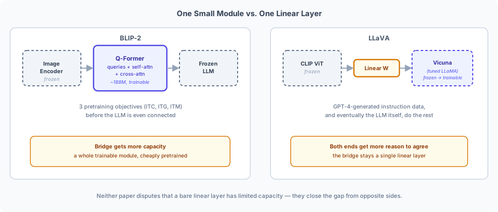
BLIP-2 closed with a question: is the Q-Former's three-objective pretraining actually necessary, or would a single trained linear layer plus instruction-tuned data do the same job? LLaVA [1] is the paper that asks that question directly, and answers it with the simplest bridge imaginable. Where BLIP-2 puts a ~188M-parameter module with its own self-attention, cross-attention, and three separately-masked pretraining objectives between a frozen image encoder and a frozen LLM, LLaVA puts one matrix multiply. No queries, no compression, no cross-attention. The vision encoder's patch features get projected, token for token, straight into the language model's embedding space, and the language model reads them exactly the way it reads any other word.

That sounds like it should work worse, not better. The Q-Former exists because BLIP-2 [6] argued a bare linear layer has too little capacity to close the gap between "pixel statistics" and "word meaning" on its own. LLaVA doesn't refute that argument — it routes around it. Instead of buying capacity with a bigger bridge, LLaVA buys it with better data: a new instruction-following dataset. An image's caption and bounding boxes — a symbolic description of the image, not the image itself — get fed as plain text to GPT-4, which never sees the pixels, and GPT-4 writes multi-turn conversations about the image from that description alone (Data Is the New Machinery, below, covers exactly how). The result is large and varied enough that a single linear layer, followed by actually fine-tuning the language model itself, turns out to be enough.

Side-by-side comparison of BLIP-2's Q-Former bridge and LLaVA's single linear-layer bridge between a frozen vision encoder and Vicuna, an instruction-tuned LLaMA — Figure 1. BLIP-2 bridges a frozen image encoder and a frozen LLM with an entire trainable module, the Q-Former. LLaVA bridges the same kind of gap with a single linear layer, and later trains the language model itself — Vicuna, an instruction-tuned variant of LLaMA — instead of giving the bridge more capacity.

This post assumes you've read ViT (the patch grid a vision transformer produces), CLIP (the specific frozen vision encoder LLaVA reuses), BLIP-2 (the bridging problem this post's opening section, From a Bootstrapped Bridge to a Single Linear Layer, argues LLaVA sidesteps rather than solves), and the decoder post (the next-token generative loss, reused directly below). None of those are re-derived here — what follows covers only what LLaVA adds on top.

From a Bootstrapped Bridge to a Single Linear Layer — why LLaVA trades the Q-Former's capacity for something else entirely
The Architecture: Three Pieces, One New Layer — a frozen CLIP encoder, one trainable projection, and a language model that eventually stops being frozen too
The Projection: Every Patch Becomes a Token — no compression, no queries, and why the visual sequence length scales with image resolution
Data Is the New Machinery — turning captions and bounding boxes into conversations a text-only GPT-4 could never have seen the pixels for
Assembling One Training Example — visual tokens, a conversation template, and where the image actually sits in the sequence
The Masked Instruction-Tuning Loss — why the model is never trained to predict its own question
Two Stages: Alignment, Then Instruction Tuning — what stays frozen, and what starts moving, in each stage
What LLaVA Buys You, and What It Costs — trainable parameter counts against BLIP-2, and the token-count bill nobody sends you until later
Putting It All Together — a minimal reference implementation of everything above, both stages

1. From a Bootstrapped Bridge to a Single Linear Layer

1.1. The argument LLaVA doesn't refute

The Bridging Problem section of the BLIP-2 post laid out why a bare linear layer struggles to bridge a frozen image encoder and a frozen LLM: the LLM's embedding space was shaped entirely by pretraining on text tokens, and a raw image feature vector, pushed through one freshly initialized projection, has no reason to land anywhere the LLM's frozen weights know how to interpret. BLIP-2's fix was to insert something with more capacity in front of that projection — the Q-Former — and pretrain it first, cheaply, before ever touching the expensive frozen LLM. Nothing about that reasoning was wrong, and LLaVA doesn't claim otherwise.

1.2. Two ways to close a capacity gap

There are two ways to make a bridge that's short on capacity actually work: give the bridge more capacity, or give the two ends more reason to already agree. BLIP-2 takes the first path. LLaVA takes the second: instead of a module that learns to translate between two mismatched representations, LLaVA trains the language model itself — not just the bridge — to expect visual tokens where it once only expected words. The projection stays a single linear layer, exactly as capacity-limited as the one BLIP-2 argued against, for the entire time the vision encoder and language model are both still frozen. What changes the outcome is what happens once they stop being frozen, covered below in The Masked Instruction-Tuning Loss and Two Stages: Alignment, Then Instruction Tuning.

1.3. What has to be true for the second path to work

Fine-tuning the LLM itself is normally the expensive part BLIP-2 was built to avoid. LLaVA accepts that cost, but only in a second stage, after a cheap first stage has already gotten the projection roughly aligned — and it only accepts that cost because Vicuna [2], the LLM LLaVA actually uses, is small enough (7B or 13B parameters) and open enough to fine-tune directly, unlike the black-box, API-only large language models BLIP-2 had reason to keep frozen. The other thing that has to be true is that there's enough of the right kind of data to make full fine-tuning teach the model something durable rather than just overfitting — and that's what Data Is the New Machinery, next, is actually about.

2. The Architecture: Three Pieces, One New Layer

Three components, and only one of them is new:

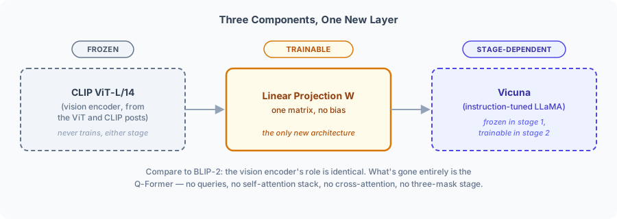
Diagram of LLaVA's three components: a frozen CLIP ViT-L/14 vision encoder, a trainable linear projection, and Vicuna, frozen in stage 1 and trainable in stage 2 — Figure 2. Three components, one of them new. The vision encoder never trains, in either stage. The projection is the only thing stage 1 ever touches. Vicuna is frozen in stage 1 and trainable in stage 2 — the one box whose label changes partway through this post.

The vision encoder is CLIP's ViT-L/14 image tower [7] [8], the exact frozen encoder the ViT post already derived, pretrained by CLIP's contrastive objective and never updated again in either of LLaVA's own training stages. The projection is one trainable linear layer, covered in full in the next section, The Projection: Every Patch Becomes a Token. The language model is Vicuna, an instruction-tuned variant of LLaMA [3] — frozen in stage 1, trainable in stage 2, the one piece of this diagram whose "frozen" label doesn't hold for the whole pipeline's lifetime.

Note: it's worth being explicit about what LLaVA reuses versus discards from BLIP-2's pipeline. The frozen vision encoder's role is identical in both papers. What's gone entirely is the Q-Former: no queries, no self-attention stack borrowed from BERT, no cross-attention, and no three-mask pretraining stage. One linear layer sits where BLIP-2 put an entire trainable transformer module.

3. The Projection: Every Patch Becomes a Token

3.1. No pooling, no compression

BLIP-2's Q-Former reads the frozen image encoder's entire patch sequence through cross-attention, but writes out a small, fixed number of query outputs — 32 in the real paper — regardless of how many patches went in. LLaVA does the opposite: every patch token that comes out of the vision encoder gets its own projected output token. Nothing gets compressed, and nothing gets thrown away.

N = (\frac{H}{P}) \times (\frac{W}{P}) (1)

For CLIP's ViT-L/14 at its native $224 \times 224$ input resolution, patch size $P = 14$ , that's $N = 16 \times 16 = 256$ patch tokens per image — a sequence length that grows with image resolution, not a constant the architecture fixes in advance the way BLIP-2's 32 queries do.

3.2. One matrix, applied to every patch

The projection itself is a single trainable matrix $W$ , with no bias term — the simplest possible linear map, applied identically to every patch:

H_{v} = Z_{v} W (2)

Concretely, for CLIP ViT-L/14 feeding Vicuna, $W \in R^{1024 \times 4096}$ : 1024 is ViT-L/14's patch feature dimension, 4096 is the dimension Vicuna's own word embeddings live in. Neither number is fixed by LLaVA's architecture — they're just this pairing's numbers; a different vision encoder or a different LLM would give $W$ different dimensions on either side.

$Z_{v}$ is the vision encoder's patch feature sequence — and specifically, excluding the [CLS] token. ViT's [CLS] token and BLIP-2's cross-attention source both kept [CLS] in play, since both needed a single pooled summary or a full sequence to attend into. LLaVA needs neither: it wants exactly the per-patch, spatially-grounded features [CLS] was never meant to carry, so [CLS] is dropped before $W$ ever sees anything — the same shape of operation as every projection this series has already used, just with nothing else attached to it.

3.3. Worked example: four patches, no `[CLS]`

Reusing ViT's toy image one more time, minus its [CLS] row this time:

Position	Patch Feature ( $Z_{v}$ )
patch 1	`[0.5, 0.9, 0.5, 0.7]`
patch 2	`[1.1, 1.4, 1.2, 1.3]`
patch 3	`[1.6, 1.3, 1.4, 1.5]`
patch 4	`[0.8, 0.6, 0.8, 0.8]`

A toy $4 \times 4$ projection matrix, standing in for the real $1024 \times 4096$ one:

import numpy as np

def softmax(x, axis=-1):
    x = x - np.max(x, axis=axis, keepdims=True)
    e = np.exp(x)
    return e / np.sum(e, axis=axis, keepdims=True)

Z_v = np.array([
    [0.5, 0.9, 0.5, 0.7],  # patch 1
    [1.1, 1.4, 1.2, 1.3],  # patch 2
    [1.6, 1.3, 1.4, 1.5],  # patch 3
    [0.8, 0.6, 0.8, 0.8],  # patch 4
])
W = np.array([
    [0.3, 0.1, -0.2, 0.4],
    [0.2, 0.5, 0.1, -0.1],
    [-0.1, 0.2, 0.4, 0.3],
    [0.4, -0.1, 0.3, 0.2],
])

H_v = Z_v @ W  # equation 2 -- no bias term, no queries, no cross-attention
print(np.round(H_v, 3))
# [[0.19  0.59  0.28  0.30]
#  [0.35  1.02  0.60  0.61]
#  [0.43  1.14  0.75  0.76]
#  [0.24  0.62  0.42  0.42]]

H_{v} = 0.190 0.350 0.430 0.240 0.590 1.020 1.140 0.620 0.280 0.600 0.750 0.420 0.300 0.610 0.760 0.420 (3)

Four patches in, four visual tokens out — $h_{v, 1}, \dots, h_{v, 4}$ , one per row above. Compare this to BLIP-2's soft-prompt projection, Equation (12), which also projects into an LLM's embedding dimension with one linear layer: the arithmetic is identical in shape, but BLIP-2's $Z$ going in already had two entries — the Q-Former's query outputs, already compressed from five frozen positions down to two, by cross-attention, before this kind of projection ever ran. Here, $Z_{v}$ going in is the frozen features themselves, and the row count of $H_{v}$ is exactly the row count of $Z_{v}$ — What LLaVA Buys You, and What It Costs, near the end of this post, comes back to that cost.

4. Data Is the New Machinery

4.1. The bridge got simpler; the data had to get harder

The previous section, The Projection: Every Patch Becomes a Token, covered the entirety of what's architecturally new in LLaVA — one matrix. Everything that makes that matrix, plus a fine-tuned LLM behind it, actually work is a data problem instead of an architecture problem, and that's most of what the LLaVA paper is actually about.

Diagram showing an image's caption and bounding boxes feeding a text-only GPT-4, which produces three types of instruction-following data: conversations, detailed descriptions, and complex reasoning — Figure 3. A text-only GPT-4 never sees the image itself — only its existing caption and a list of bounding boxes. From that symbolic description alone, three different prompts produce three different kinds of training data: conversations, detailed descriptions, and complex reasoning.

4.2. GPT-4 that has never seen the image

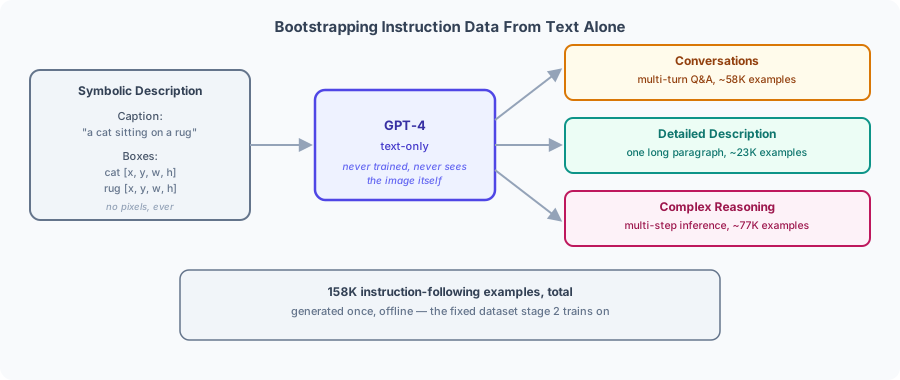
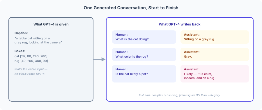
There was no large dataset of multi-turn visual conversations to train on in 2023, so LLaVA's authors built one — but the obvious way to build it, showing images to a vision-language model and asking it to generate conversations about them, wasn't available at the scale they needed with the tools that existed then. Their workaround: prompt a text-only GPT-4 [4] with a symbolic representation of an image — its existing human-written caption(s), plus a list of object categories and bounding-box coordinates, both already available for images drawn from COCO — and ask it to generate conversational data as if it could see the picture. GPT-4 never touches a pixel. Captions and boxes are the only channel information about the image travels through.

Concretely, a box is four numbers, [x, y, w, h] — its top-left corner, then its width and height, in pixels. From that alone, with no caption help, GPT-4 can work out things a caption often never bothers to state. Two boxes both labeled person, at [30, 40, 80, 200] and [220, 50, 75, 190], say there are two people, roughly the same size, sitting side by side — the second box starts well to the right of where the first one ends. None of that needs a pixel; it's ordinary arithmetic on four numbers per box. Figure 4's own cat-and-rug example below leans more on the caption than on this kind of geometry, since the caption already says the cat is "sitting on" the rug — but this same overlap-and-position arithmetic is what lets the complex-reasoning category answer questions about relative position, count, or size that no caption in the dataset spells out.

4.3. Three kinds of instruction-following data

Three different prompts to the same text-only GPT-4, over the same underlying captions and boxes, produce three distinct kinds of training example: conversations, multi-turn question-and-answer exchanges about the image, written as if a person were asking and an assistant that can see the picture were answering; detailed descriptions, a single long, thorough paragraph describing everything the boxes and captions imply is in the scene; and complex reasoning, questions whose answers require a step or two of inference beyond what's directly stated — not "what color is the object" but "why might this person be doing that," answerable only by combining several boxes and captions at once. The real dataset totals 158K such examples: roughly 58K conversations, 23K detailed descriptions, and 77K complex-reasoning instances.

Example of one generated conversation-type training instance: an image with its caption and boxes on one side, a generated multi-turn question-and-answer exchange on the other — Figure 4. One concrete instance of the pipeline in Figure 3: a caption and a handful of boxes go in, a multi-turn conversation that reads as if the assistant could see the picture comes out — written by a model that never had access to the pixels.

Note: none of this data generation happens inside the model being trained, and none of it happens more than once. It's an offline preprocessing step, run against a separate, much larger model, that produces a fixed dataset file — the same relationship BLIP's own bootstrapped captions have to the BLIP-2 pipeline that trains on them, one level removed: BLIP bootstraps data with a model it also trains; LLaVA bootstraps data with a model (GPT-4) it never trains or even has access to the weights of.

5. Assembling One Training Example

5.1. Where the visual tokens actually sit

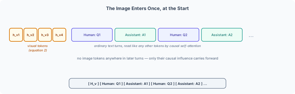
A single training example is a sequence: the projected visual tokens $H_{v}$ from The Projection: Every Patch Becomes a Token, some fixed instruction text, and a conversation — one or more turns of a human question followed by an assistant answer. The image is introduced exactly once, at the very start of the first turn, never repeated in later turns of the same conversation:

Diagram of a training sequence: projected visual tokens at the start, followed by repeated human and assistant turns — Figure 5. The projected visual tokens appear exactly once, at the very start of the sequence — never repeated in later turns of the same conversation. Every turn after that is ordinary text, read by the language model through the same causal self-attention it was already using.

5.2. A concrete sequence

Continuing the toy image from The Projection: Every Patch Becomes a Token (a cat, per the ViT and CLIP posts' running example), one training example's full token sequence, in order:

[h_v1] [h_v2] [h_v3] [h_v4]  Human: What animal is in this photo?  Assistant: a cat <EOS>

$h_{v 1}, \dots, h_{v 4}$ are the four rows of $H_{v}$ from Equation (3) — continuous vectors, not lookups into a fixed embedding table, the identical "soft" role BLIP-2's projected query outputs played once they were prepended to a caption. Every other token in this sequence — Human:, the question text, Assistant:, the answer, <EOS> — is an ordinary token, looked up from Vicuna's own embedding table exactly as if this were a plain text conversation.

5.3. Multiple turns, one image

Real training examples from the conversation-type data have several human/assistant turn pairs, not just one. The visual tokens still appear only at the start, exactly as in the diagram above:

[h_v1]...[h_v4]  Human: Q1  Assistant: A1  Human: Q2  Assistant: A2  Human: Q3  Assistant: A3

Every later turn's assistant answer can, in principle, depend on the visual tokens from the very start of the sequence — ordinary causal self-attention reaches all the way back, the identical reasoning the decoder post's own causal masking already established for why position $i$ can attend to any position $j \leq i$ , regardless of how far back $j$ is.

6. The Masked Instruction-Tuning Loss

6.1. The same next-token loss, with one new rule

The sequence from Assembling One Training Example is generated left to right, one token predicting the next, exactly the mechanism the decoder post's training objective already covers:

P (x_{1}, \dots, x_{L}) = i = 1 \prod L P (x_{i} ∣ x_{< i}) (4)

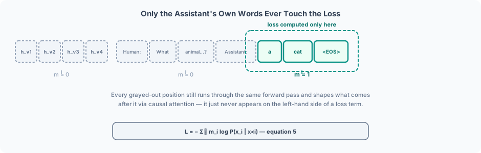
Naively summing $- lo g P (x_{i} ∣ x_{< i})$ over every position $i$ , the way BLIP-2's ITG and stage-2 losses both do over their target captions, would also train the model to predict the human's own question — What, then animal, then is, and so on — as if generating a plausible-sounding question were the point. It isn't. The fix is a per-token mask:

L = - i = 1 \sum L m_{i} lo g P (x_{i} ∣ x_{< i}), m_{i} = {10 x_{i} is part of an assistant answer otherwise (5)

$m_{i} = 0$ for the visual tokens, the Human:/Assistant: template markers, and the question text itself — all of that still sits in $x_{< i}$ , still shapes every prediction that follows it through ordinary causal attention, but never once appears on the left-hand side of a loss term. Only $m_{i} = 1$ positions — the assistant's actual answer tokens, plus the <EOS> that ends each one — ever get compared against a target and backpropagated.

Diagram of a token sequence with the visual tokens, human question, and template markers grayed out, and only the assistant's answer tokens highlighted as contributing to the loss — Figure 6. Every position still produces a prediction, and every position still shapes what comes after it through causal attention — but only the highlighted assistant-answer positions ever appear in the loss. The model is never rewarded or penalized for how well it predicts its own question.

6.2. Worked example: predicting "cat"

Reusing BLIP-2's own stage-2 worked example almost exactly — same toy vocabulary, same hidden-state stand-in, same vocabulary projection — since the mechanism computing a single next-token probability hasn't changed at all; what's different here is only which positions in the full sequence this computation is ever allowed to run for:

vocab = ["a", "photo", "of", "cat", "dog", "bird", "car", "<EOS>"]
h_gen = np.array([0.9, 0.3, 0.1, 0.1])  # hidden state at the position predicting "cat"

W_vocab = np.array([
    [0.1, 0.1, 0.1, 0.5, -0.2, -0.1, -0.2, -0.1],
    [0.1, 0.2, 0.1, 0.3, 0.1, -0.1, -0.1, -0.2],
    [-0.1, 0.1, 0.2, 0.2, 0.1, 0.1, -0.1, 0.3],
    [0.2, -0.1, 0.1, 0.2, -0.2, 0.1, 0.2, 0.2],
])
b_vocab = np.array([0.1, 0.1, 0.1, 0.1, 0.1, 0.1, 0.1, -0.2])

logits = h_gen @ W_vocab + b_vocab
probs = softmax(logits)
print(vocab[np.argmax(probs)], round(probs.max(), 3))
# cat 0.211

loss_this_position = -np.log(probs[vocab.index("cat")])
print(round(loss_this_position, 3))
# 1.559

P ("cat" ∣ H_{v}, "Human: What animal is in this photo? Assistant: a") m_{i} \approx 0.211 = 1 here (6)

The position predicting What (the second token of the human's question) would run through the identical softmax machinery, over the identical vocabulary, conditioned on everything before it — but $m_{i} = 0$ there, so whatever probability the model assigns What never contributes a term to Equation (5) at all. Nothing about the forward pass changes at that position; only whether its output is ever looked at by the loss does.

6.3. Multi-turn: sum over turns, same rule inside each

For a full multi-turn conversation, Equation (5) just sums across every turn's assistant tokens, one flat loss over the whole sequence rather than one loss per turn:

L = - t = 1 \sum T i \in turn t ’s answer \sum lo g P (x_{i} ∣ x_{< i}) (7)

Every human turn, at every $t$ , still contributes exactly zero loss terms — $m_{i} = 0$ inside every one of them, the same rule as the single-turn case, just applied $T$ times instead of once.

7. Two Stages: Alignment, Then Instruction Tuning

Diagram comparing stage 1 (vision encoder and LLM frozen, only the projection trains) and stage 2 (vision encoder frozen, projection and LLM both train) — Figure 7. Stage 1 trains only the projection, against a simple one-turn caption task, while both large models stay frozen. Stage 2 keeps the vision encoder frozen but lets the projection and the entire language model train together, against the full instruction-following dataset.

7.1. Stage 1 — pre-training for feature alignment

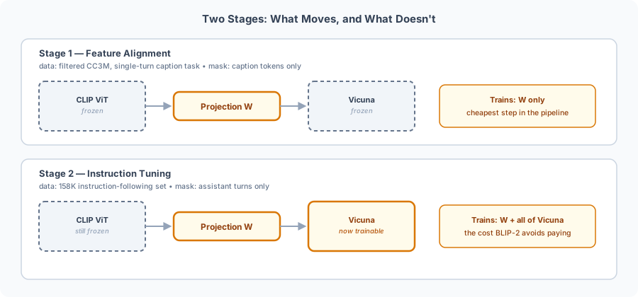
Stage 1 freezes both the vision encoder and the language model, training only the projection $W$ — the smallest possible set of trainable parameters in this whole pipeline, the identical "train the bridge first, cheaply" logic BLIP-2's stage 1 already used, even though the bridge itself is architecturally nothing alike. The data here isn't the 158K instruction-following set from Data Is the New Machinery — it's a filtered 595K-example subset of CC3M [5], each example a single (image, caption) pair reformatted as a one-turn "question, answer" exchange: a generic instruction like "Describe the image" as the human turn, the existing caption as the entire assistant answer. Equation (5)'s mask applies here too — only the caption tokens, standing in for the assistant's answer, ever contribute to the loss. By the end of stage 1, $W$ has learned to place visual tokens somewhere in Vicuna's embedding space that a frozen Vicuna already finds usable, without either large model moving an inch.

7.2. Stage 2 — fine-tuning end to end

Stage 2 keeps the vision encoder frozen — it never trains in either stage, in the real paper — but now updates both $W$ and the language model itself, training on the full 158K instruction-following dataset from Data Is the New Machinery, mixing conversations, detailed descriptions, and complex reasoning examples together in one training run. This is the step that costs what BLIP-2 was built to avoid: an actual forward-and-backward pass through billions of language model parameters, every training step. It's also the step that does the real work From a Bootstrapped Bridge to a Single Linear Layer promised — by training the LLM to expect visual tokens rather than just training a translator to speak the LLM's existing language, the model as a whole gets to close the modality gap BLIP-2's Bridging Problem section worried about, from both sides at once, not just the vision side.

7.3. Why the order matters

Running stage 2 without stage 1 first would start $W$ from random weights while simultaneously asking the LLM to adapt to whatever nonsense $W$ initially produces — a much harder joint optimization problem, and closer to CLIP's own from-scratch joint training than to anything LLaVA is trying to be cheaper than. Stage 1 exists so that stage 2 starts from visual tokens that are already roughly in the right neighborhood, leaving stage 2 to refine rather than discover that alignment from nothing.

8. What LLaVA Buys You, and What It Costs

8.1. Trainable parameters, against BLIP-2

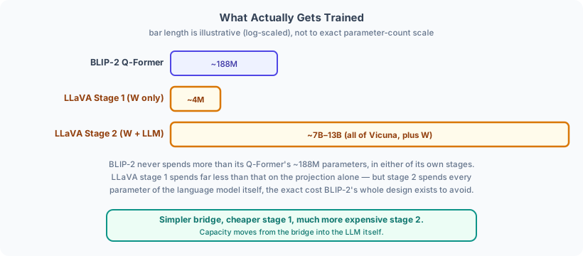
Bar comparison of parameters trained by BLIP-2's Q-Former, LLaVA stage 1's projection, and LLaVA stage 2's projection plus full language model — Figure 8. BLIP-2 never trains more than its ~188M-parameter Q-Former. LLaVA stage 1 trains far less than that — just the projection — but stage 2 trains the entire language model on top of it, billions of parameters BLIP-2's whole design was built to avoid touching.

Stage 1 trains only $W$ — a few million parameters, smaller even than BLIP-2's ~188M-parameter Q-Former. Stage 2 trains $W$ plus the entire language model — 7B or 13B parameters, every one of them, dwarfing anything either paper trains in any other stage. BLIP-2's whole pitch was never spending that cost; LLaVA spends it once, deliberately, in exchange for not needing a bespoke bridge module at all.

8.2. The bill nobody sends you until later

The Projection: Every Patch Becomes a Token's equation 1 already flagged where the other cost hides: $N = 256$ visual tokens per image at LLaVA's resolution, every one of them a full position in the language model's sequence, attended to and attending like any other token. BLIP-2's Q-Former fixes this at a constant 32 regardless of image size — more architecture, but a flat, predictable context-length cost. LLaVA's context-length cost scales directly with image resolution, and grows further, un-amortized, with every additional image or higher-resolution input a later system wants to support. Trading the Q-Former's capacity for a linear layer was From a Bootstrapped Bridge to a Single Linear Layer's story; this is the other half of that trade, paid at inference time rather than training time.

8.3. Where this leads

Nothing in this post's mechanism is new by itself: ViT's patch grid, CLIP's frozen encoder, and the decoder post's next-token loss are all reused exactly as earlier posts left them. What's new is the combination — one linear layer instead of a bridging module, a per-token loss mask instead of supervising an entire sequence, and a GPT-4-bootstrapped instruction dataset standing in for everything the Q-Former's three pretraining objectives used to buy. LLaVA-1.5 [9] pushes on exactly the two costs this section just raised: a two-layer MLP in place of the single linear projection, and higher-resolution images handled by tiling rather than one larger encoder pass — neither of which changes anything about the masked instruction-tuning loss this post derived above.

9. Putting It All Together

9.1. Scope: what's novel here, and what's assumed

Everything below is LLaVA-specific: the projection, the sequence assembly, the masked loss, and the two training stages. Standard building blocks this series already covered elsewhere — tokenization, the frozen vision transformer, and the causal transformer decoder itself — are left as stubs with a docstring pointing at where they actually get built. This is architecture-level reference code: it shows the real data flow and the real shapes, but frozen_clip_vit and vicuna_forward are undefined, so unlike the toy snippets earlier in this post, it isn't something you can paste and run.

import numpy as np

def softmax(x, axis=-1):
    e = np.exp(x - np.max(x, axis=axis, keepdims=True))
    return e / np.sum(e, axis=axis, keepdims=True)

def frozen_clip_vit(images):
    """Frozen in both stages -- see The Architecture: Three Pieces, One New
    Layer. Returns Z_v, the patch feature sequence with [CLS] already
    dropped (equation 2)."""
    ...

def vicuna_forward(input_embeds, target_ids=None):
    """The language model. Frozen in stage 1, trainable in stage 2 (see Two
    Stages: Alignment, Then Instruction Tuning). Returns per-position logits
    over Vicuna's vocabulary."""
    ...

def tokenize_and_embed(text, embedding_table):
    """Ordinary lookup into Vicuna's own word embedding table -- everything
    in a training sequence that isn't a projected visual token."""
    ...

9.2. The projection

One matrix, no bias, applied to every patch token (equation 2):

def project_visual_tokens(Z_v, W):
    """H_v = Z_v @ W -- equation 2. No queries, no cross-attention, no
    compression: len(H_v) == len(Z_v) always."""
    return Z_v @ W

9.3. Assembling one training example

Visual tokens once, at the start; every other turn is ordinary text (see Assembling One Training Example):

def build_sequence(H_v, turns, embedding_table):
    """turns: list of (human_text, assistant_text) pairs, in order. Returns
    the full embedding sequence and a same-length boolean mask, m_i in
    equation 5 -- True only where a loss term is ever computed."""
    embeds = [H_v]                     # image tokens, once, at the very start
    mask = [False] * len(H_v)

    for human_text, assistant_text in turns:
        human_embeds = tokenize_and_embed(f"Human: {human_text} Assistant:", embedding_table)
        answer_embeds = tokenize_and_embed(f" {assistant_text} <EOS>", embedding_table)

        embeds += [human_embeds, answer_embeds]
        mask += [False] * len(human_embeds)   # question + template: never supervised
        mask += [True] * len(answer_embeds)   # the assistant's own words: supervised

    return np.concatenate(embeds, axis=0), np.array(mask)

9.4. The masked loss

Reads only the positions build_sequence marked True (equations 5 and 7):

def masked_lm_loss(logits, target_ids, mask):
    """logits: (L, vocab_size), one row per sequence position. Sums
    -log P(target_i | x_<i) only where mask[i] is True; every other
    position's prediction is computed but never touches the loss."""
    log_probs = np.log(softmax(logits, axis=-1))
    per_position_loss = -log_probs[np.arange(len(target_ids)), target_ids]
    return np.sum(per_position_loss * mask)

9.5. Stage 1: freeze everything but the projection

def stage1_step(batch, W, embedding_table):
    Z_v = frozen_clip_vit(batch.images)         # frozen throughout both stages
    H_v = project_visual_tokens(Z_v, W)         # the only thing this stage trains

    # Stage 1's "conversation" is always one turn: a generic instruction, the
    # image's own caption as the entire assistant answer.
    seq, mask = build_sequence(H_v, [("Describe the image.", batch.caption)], embedding_table)
    logits = vicuna_forward(seq)                # Vicuna's own weights: frozen this stage

    loss = masked_lm_loss(logits, batch.target_ids, mask)
    loss.backward()   # gradient reaches W only -- frozen_clip_vit and vicuna_forward get none
    optimizer.step()

9.6. Stage 2: fine-tune the projection and the language model together

def stage2_step(batch, W, embedding_table):
    Z_v = frozen_clip_vit(batch.images)         # still frozen -- never trains, in either stage
    H_v = project_visual_tokens(Z_v, W)

    # Stage 2's turns come from the 158K instruction-following dataset --
    # conversations, detailed descriptions, and complex reasoning, mixed together.
    seq, mask = build_sequence(H_v, batch.turns, embedding_table)
    logits = vicuna_forward(seq)                # Vicuna's own weights: trainable this stage

    loss = masked_lm_loss(logits, batch.target_ids, mask)
    loss.backward()   # gradient reaches both W and every Vicuna parameter
    optimizer.step()

That's the entire system: one projection, reused unmodified between both stages; one sequence builder and one masked loss, shared by both; and the only thing that changes between stage1_step and stage2_step is which parameters optimizer.step() is actually allowed to move.

References

[1]Liu, Li, Wu & Lee (2023). Visual Instruction Tuning. Neural Information Processing Systems (NeurIPS).
[2]Chiang et al. (2023). Vicuna: An Open-Source Chatbot Impressing GPT-4 with 90%* ChatGPT Quality. LMSYS Org (blog).
[3]Touvron et al. (2023). LLaMA: Open and Efficient Foundation Language Models.
[4]OpenAI (2023). GPT-4 Technical Report.
[5]Sharma, Ding, Goodman & Soricut (2018). Conceptual Captions: A Cleaned, Hypernymed, Image Alt-text Dataset For Automatic Image Captioning. Association for Computational Linguistics (ACL).
[6]Li, Li, Savarese & Hoi (2023). BLIP-2: Bootstrapping Language-Image Pre-training with Frozen Image Encoders and Large Language Models. International Conference on Machine Learning (ICML).
[7]Radford et al. (2021). Learning Transferable Visual Models From Natural Language Supervision. International Conference on Machine Learning (ICML).
[8]Dosovitskiy et al. (2020). An Image is Worth 16x16 Words: Transformers for Image Recognition at Scale. International Conference on Learning Representations (ICLR).
[9]Liu, Li, Li & Lee (2023). Improved Baselines with Visual Instruction Tuning.

LLaVA: Visual Instruction Tuning

Contents