CLIP trains two towers, an image encoder and a text encoder, from scratch, together, on hundreds of millions of pairs. That works, but it's expensive — every improvement to either tower means paying that joint training cost again. BLIP-2 [1] takes its name, and its core idea, from its predecessor, BLIP [2] — "bootstrapping" a vision-language model rather than training one from a blank slate. The original BLIP bootstrapped its training data, filtering and re-captioning noisy web image-text pairs with a jointly trained model of its own. BLIP-2 bootstraps something more structural: by the time it was published, excellent frozen image encoders already existed, and so did large language models capable of writing fluent, coherent text about almost anything — except what's in a picture, since none of them had ever seen one. The question BLIP-2 asks is deceptively simple: instead of training a vision-language model from scratch, can you just wire two already-trained, unimodal models together — freeze both, train almost nothing?
The answer needs one new piece of machinery, the Querying Transformer, or Q-Former — a small module sitting between the frozen image encoder and the frozen language model, built almost entirely out of parts this series has already derived. Its self-attention layers are initialized from BERT. Its cross-attention layers are the exact mechanism from the decoder post, just reaching into a frozen source instead of a jointly trained one. Its first pretraining objective is CLIP's own contrastive loss, reused almost verbatim. What's genuinely new is how those pieces get combined — a small set of learnable query tokens, trained with three different objectives at once by changing nothing but which attention mask is applied to the same shared weights — and what that buys: a single small module, trained cheaply, that makes two large, expensive, never-retouched models usable together.
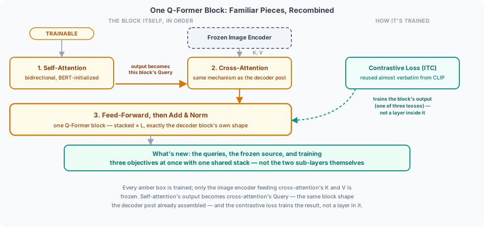
This post assumes you've read ViT (the frozen image encoder), BERT
(the Q-Former's self-attention initialization and its [CLS]-style readout), the decoder post
(cross-attention), and CLIP (the contrastive loss and its toy batch, reused
directly below). None of those are re-derived here — what follows covers only what BLIP-2 adds on top.
Contents
- The Bridging Problem — why freezing two large pretrained models and connecting them isn't as simple as one linear layer
- The Q-Former: Queries and Cross-Attention — learnable query tokens, a shared self-attention stack, and cross-attention into a frozen image encoder
- Stage 1, Loss 1 — Image-Text Contrastive (ITC) — the unimodal mask, max-over-queries pooling, and CLIP's own contrastive math
- Stage 1, Loss 2 — Image-Grounded Text Generation (ITG) — the multimodal causal mask, forcing the queries to carry everything a caption needs
- Stage 1, Loss 3 — Image-Text Matching (ITM) — the bidirectional mask and an averaged-over-queries classifier
- One Shared Stack, Three Masks — why all three losses can't come from a single forward pass, unlike BERT's MLM and NSP
- Stage 2 — Bridging to a Frozen LLM — projecting query outputs into soft prompt tokens and a generative loss
- What BLIP-2 Buys You — trainable parameter counts, and what comes next
- Putting It All Together — a minimal reference implementation of everything above, both stages
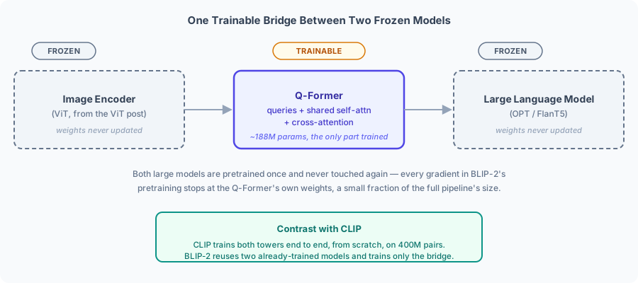
1. The Bridging Problem
1.1. Two expensive models, already trained
By 2023, a frozen ViT-scale image encoder and a frozen large language model were each, independently, the product of an enormous training run — ViT-style encoders pretrained on hundreds of millions of images, LLMs pretrained on web-scale text. Retraining either one from scratch just to make them work together, the way CLIP trains its two towers jointly, throws away all of that. The obvious alternative: freeze both, and find some small, cheap-to-train piece that translates between them.
1.2. Why a single linear layer struggles
The naive version of that idea is one linear layer: project the image encoder's output straight into the LLM's embedding dimension, feed it in as if it were a couple of extra "words," and train only that projection against the LLM's ordinary generative loss. The dimension mismatch is trivial to fix — it's just a matmul, the same shape of operation as every , , or already used in this series. The harder problem is underneath that: the LLM's embedding space was shaped entirely by pretraining on text tokens. A raw image feature vector, pushed through one freshly initialized linear layer, has no reason to land anywhere the LLM's frozen weights know how to interpret — there's a wide modality gap between "a sequence of patches encoding pixel statistics" and "a sequence of tokens encoding word meaning," and one linear layer, trained only against the LLM's downstream loss, has comparatively little capacity to close it.
1.3. BLIP-2's answer: a small module with real capacity, pretrained first
BLIP-2's fix is to put something with more capacity than a bare linear layer in front of that projection — the Q-Former — and to pretrain it first, cheaply, against objectives that don't require the expensive frozen LLM at all. Only once the Q-Former has already learned to extract visual features that are well-organized and language-adjacent does it get connected to the LLM, at which point bridging the remaining gap is a much smaller job. The rest of this post covers exactly that: what the Q-Former is (module 2), the three cheap objectives that pretrain it (modules 3-5), and the final, much smaller step of connecting it to a frozen LLM (module 7).
2. The Q-Former: Queries and Cross-Attention
The modules ahead build this up one piece at a time, and each piece gets its own figure — which makes it easy to lose the forest for the trees. Before any of that, here's the whole thing at once: the architecture, bottom-up, and all three pretraining objectives reading off its outputs, the same way the original BLIP-2 paper's own architecture figure lays it out.
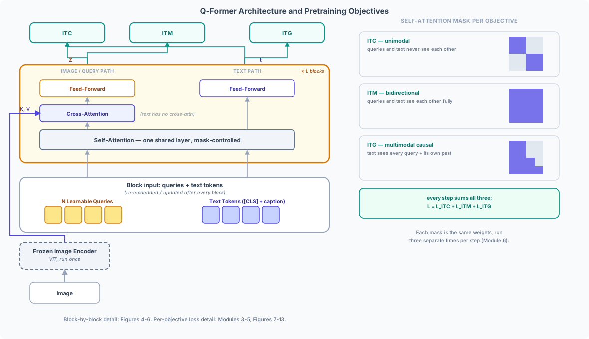
Everything below this point is one of two things: either it's deriving a piece of the block in the middle (modules 2 and — via Figures 4-6 — the exact self-attention/cross-attention/FFN shape), or it's walking through one of the three mask panels on the right in detail (modules 3-5). Nothing past this point introduces a fourth piece that isn't already sitting somewhere in this figure.
2.1. From one [CLS] token to many query tokens
ViT's [CLS] token and CLIP's [EOS] token both
solved the same problem the same way: prepend (or append) one extra learnable token, let it gather
information from the whole sequence through self-attention, and read a single summary vector back out of it.
The Q-Former generalizes that trick from one dedicated token to a small set of them — 32 learnable query
embeddings in the real paper, reduced to 2 for this post's toy example, purely to keep the arithmetic
readable by hand. Each query starts as a plain trainable vector, exactly like [CLS] did, with no fixed
meaning before training begins.
2.2. Two submodules, one shared self-attention stack
The Q-Former is really two submodules wired together: an image transformer and a text transformer, both built from the same stack of self-attention layers, initialized from a pretrained BERT [3] — the identical bidirectional self-attention the BERT post's Transformer Encoder module already covered, reused as a starting point rather than trained from random weights. The image transformer additionally has cross-attention layers, inserted every other block, that reach into the frozen image encoder's output — the one piece of the Q-Former that has no BERT equivalent to initialize from, so it starts randomly. The text transformer has no cross-attention layers at all; it only ever reads the frozen image encoder through the queries, a point module 4 leans on directly.
Note: "image transformer" is the Q-Former's own name for this submodule — it is not another name for ViT, and it's worth being deliberate about keeping the two apart. ViT has already finished its entire job, completely on its own, before any of this runs: patchify, embed, prepend
[CLS], add positional embeddings, run through its own encoder blocks, and hand back one finished output sequence — exactly that post's pipeline, unmodified, with no queries involved anywhere in it. The image transformer, despite the name, never sees a raw pixel or a patch. The only image-related thing it ever touches is that single, already-finished frozen sequence, and only through cross-attention — covered next.
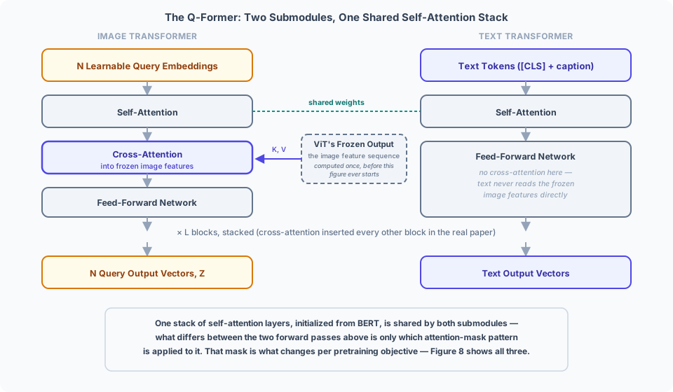
Note: Figure 4 draws two separate boxes for the two self-attention passes, which is the right picture only when the mask keeps queries and text apart entirely — ITC's case, covered next. "Shared weights" means something stronger than two independent computations that happen to use the same matrices: depending on the mask, queries and text tokens get concatenated into one combined sequence and run through a single self-attention pass together, and it's the mask alone — not the architecture — that decides whether a query position is allowed to see a text position. ITG and ITM (modules 4 and 5) both depend on exactly this: text attending to queries only works because they were in the same sequence to begin with. Module 6 lines up all three masks side by side.
2.3. The full stack: both rows, every block
Figure 4 draws a single representative block in detail — but "N Learnable Query Embeddings" and "Text Tokens" at the top of that figure are only ever block 1's input. Every block after that receives whatever the previous block produced, the identical stacking convention the encoder post's own blocks already used: block 5 has no idea what block 2 learned, and neither row reaches back for the original input a second time. Cross-attention alternates on the image row only — block 1 has it, block 2 doesn't, block 3 does again, up to block . The text row's own shape never changes: self-attention (shared with the image row, mask permitting) plus its own feed-forward network, every single block, cross-attention or not. It's easy to read "cross-attention alternates" as "the text row sits out every other block" — it doesn't; cross-attention is the one sub-layer text never gets, in any block, not a sub-layer it only skips sometimes:
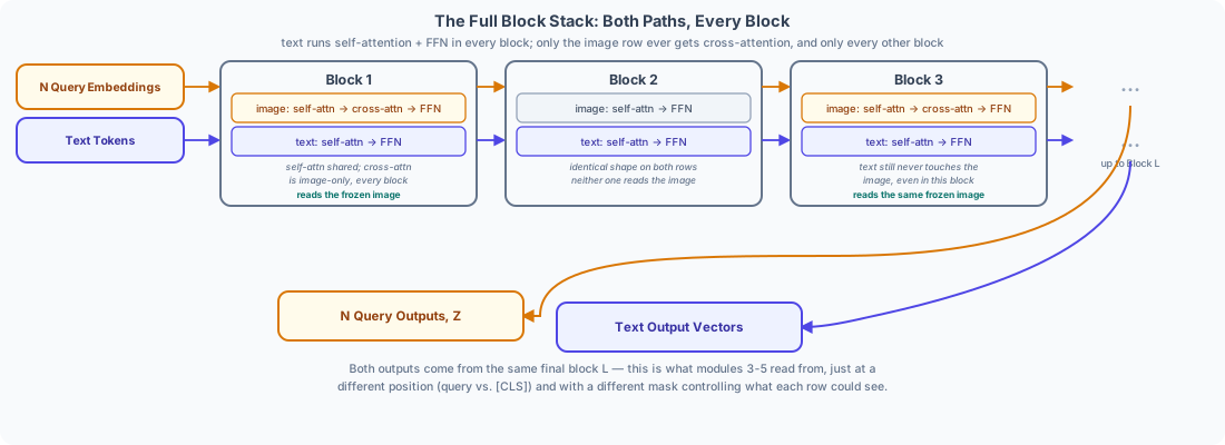
Every cross-attention occurrence, on the image row, reads the exact same — the frozen image encoder never runs a second time, and block 3 doesn't see a transformed version of the image, or block 1's already-computed output. What's different is the projection: block 3 has its own, separately-learned and , so it looks at that identical frozen sequence through its own lens rather than reusing block 1's and — the same convention the decoder post's Cross-Attention module already established for a plain encoder-decoder stack, where every decoder block's cross-attention reads the same encoder output , each through its own weights. The query side is what actually accumulates block to block — self-attention's output at block 3 already carries forward whatever blocks 1 and 2 absorbed; itself never changes.
2.4. Cross-attention into a frozen source
The mechanism itself is exactly the decoder post's Cross-Attention module — Equation (1), from one sequence, and from another — with the decoder's role played by the queries, and the encoder's role played by the frozen image encoder:
is the frozen image encoder's full output sequence — ViT's[CLS] plus every patch token, not just the pooled [CLS] vector CLIP's image tower
read out. The Q-Former's cross-attention needs the whole sequence to have anything to select from. Nothing
about the formula changed from the decoder post's version — same
underneath, same "K and V always share a source, Q doesn't" reasoning for why this is a legal
generalization of self-attention. What's different is what that frozen source is: not a co-trained
encoder whose weights move together with the decoder's during training, the way the original
Transformer's encoder and decoder do, but a completely frozen
one, pretrained independently and never touched again.
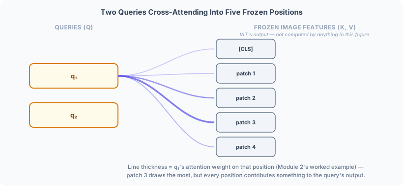
2.5. Worked example: two queries, five frozen positions
A frozen image feature sequence — [CLS] plus four patches, the familiar toy image from the ViT post, with
[CLS]'s row reused directly from that post's hypothetical classification-head input,
:
| Position | Frozen Image Feature () |
|---|---|
[CLS] | [0.4, 1.1, 0.7, 0.3] |
| patch 1 | [0.5, 0.9, 0.5, 0.7] |
| patch 2 | [1.1, 1.4, 1.2, 1.3] |
| patch 3 | [1.6, 1.3, 1.4, 1.5] |
| patch 4 | [0.8, 0.6, 0.8, 0.8] |
Two learnable queries, hand-picked starting vectors the same way ViT's [CLS] token
got one:
| Query | Starting Vector |
|---|---|
[0.2, 0.2, 0.2, 0.2] | |
[0.1, 0.3, 0.2, 0.1] |
Note: a real block runs self-attention before cross-attention — module 2's own opening point, and Figure 1's whole reason for existing. This worked example skips straight to cross-attention, projecting directly from each query's raw starting vector rather than from what self-attention would have already turned it into, the identical simplification the decoder post's own cross-attention module made for the same reason: keeping this module focused on the one new thing, cross-attention itself, rather than re-deriving self-attention's arithmetic a third time.
Projecting both queries through single-head (4x2, the same simplification the encoder
post made before introducing multiple heads), and both the frozen
positions through and — each row below is exactly one vector times one weight matrix, e.g.
patch 1's row of is patch1 @ W_K, nothing more:
| Query | (= query @ ) |
|---|---|
[0.400, 0.400] | |
[0.400, 0.300] |
| Position | (= position @ ) | (= position @ ) |
|---|---|---|
[CLS] | [1.100, 1.400] | [0.450, 0.250] |
| patch 1 | [1.000, 1.600] | [0.350, 0.475] |
| patch 2 | [2.300, 2.700] | [0.650, 0.925] |
| patch 3 | [3.000, 2.800] | [0.675, 1.150] |
| patch 4 | [1.600, 1.400] | [0.350, 0.600] |
Every one of those rows is indexed by a single query or a single position — nothing has compared a query against a position yet. is where that comparison happens, and it's why the next table has a different shape entirely: two rows (queries), five columns (positions), one scalar per pair, not one vector per row the way , , and above are:
[CLS] | patch 1 | patch 2 | patch 3 | patch 4 | |
|---|---|---|---|---|---|
| 0.707 | 0.735 | 1.414 | 1.640 | 0.849 | |
| 0.608 | 0.622 | 1.223 | 1.442 | 0.750 |
Worked out for against [CLS]: row of , [0.4, 0.4], dotted with row [CLS] of ,
[1.1, 1.4], gives ; dividing by gives
. Every other cell is the same recipe: row of dotted with row of , scaled.
Softmax across each row — one query's five scores, turned into a distribution that sums to 1 — gives each query's attention weights over the five frozen positions:
| Query | [CLS] | patch 1 | patch 2 | patch 3 | patch 4 |
|---|---|---|---|---|---|
| 0.129 | 0.133 | 0.262 | 0.328 | 0.149 | |
| 0.137 | 0.139 | 0.253 | 0.315 | 0.157 |
Both queries lean most heavily on patch 3 — the frozen position with the largest raw values — but neither one ignores the rest; every position contributes something, the same "blend of everything, weighted by relevance" behavior the encoder post's Self-Attention module first produced. Blending by these weights, then restoring through exactly the way the decoder post's Assembling a Full Decoder Block module did for its own cross-attention output:
import numpy as np

def softmax(x, axis=-1):
    x = x - np.max(x, axis=axis, keepdims=True)
    e = np.exp(x)
    return e / np.sum(e, axis=axis, keepdims=True)

H_img = np.array([
    [0.4, 1.1, 0.7, 0.3],  # [CLS]  (= ViT post's z_cls)
    [0.5, 0.9, 0.5, 0.7],  # patch 1
    [1.1, 1.4, 1.2, 1.3],  # patch 2
    [1.6, 1.3, 1.4, 1.5],  # patch 3
    [0.8, 0.6, 0.8, 0.8],  # patch 4
])
Queries = np.array([
    [0.2, 0.2, 0.2, 0.2],
    [0.1, 0.3, 0.2, 0.1],
])

W_Q = np.array([[1.0, 0], [1.0, 0], [0, 1.0], [0, 1.0]])
W_K = np.array([[1.0, 0], [0, 1.0], [1.0, 0], [0, 1.0]])
W_V = np.array([[0, 0.25], [0.25, 0], [0.25, 0], [0, 0.5]])
W_O = np.array([[1.0, 0, 1.0, 0], [0, 1.0, 0, 1.0]])

Q = Queries @ W_Q
K = H_img @ W_K
V = H_img @ W_V

d_k = K.shape[-1]
weights = softmax(Q @ K.T / np.sqrt(d_k), axis=-1)
cross_out = weights @ V
query_repr = cross_out @ W_O

print(np.round(weights, 3))
# [[0.129 0.133 0.262 0.328 0.149]
#  [0.137 0.139 0.253 0.315 0.157]]
print(np.round(query_repr, 3))
# [[0.548 0.804 0.548 0.804]
#  [0.542 0.79  0.542 0.79 ]]
In the real Q-Former, this cross-attention step is block 1's second sub-layer, not its first — self-attention runs before it, and a feed-forward network closes the block out afterward, the same three-step shape repeated across several stacked blocks. Look again at Equation (1):
— the one term that depends on which image is being processed — appears in and , but not in . For block 1's cross-attention specifically, and are both fixed, trained parameters with no anywhere upstream of them either, so
is a constant: the same matrix for every image, computable once after training and reused at inference instead of recomputed on every forward pass. and can't be cached the same way, since they're linear functions of — which is exactly why the attention weights above vary by position at all; nothing about changed, only what it was compared against.
That stops being true one layer later. Cross-attention is inserted every other block, and by the second occurrence, self-attention has already mixed the first cross-attention's image-dependent output back into the queries' own representation — so , the query for the next cross-attention layer, is a function of too, indirectly, through everything that happened in between. Only the very first cross-attention layer's gets to start from something genuinely input-independent.
The next three modules cover what those queries are actually trained to do, and it comes down entirely to one thing: which cells of the self-attention mask are open.
3. Stage 1, Loss 1 — Image-Text Contrastive (ITC)
Each of the next three modules builds up one piece at a time — the mask, the pooling, the loss — which makes it easy to lose the end-to-end shape along the way. Before any of that, here's the whole ITC computation for a single image-caption pair, start to finish:
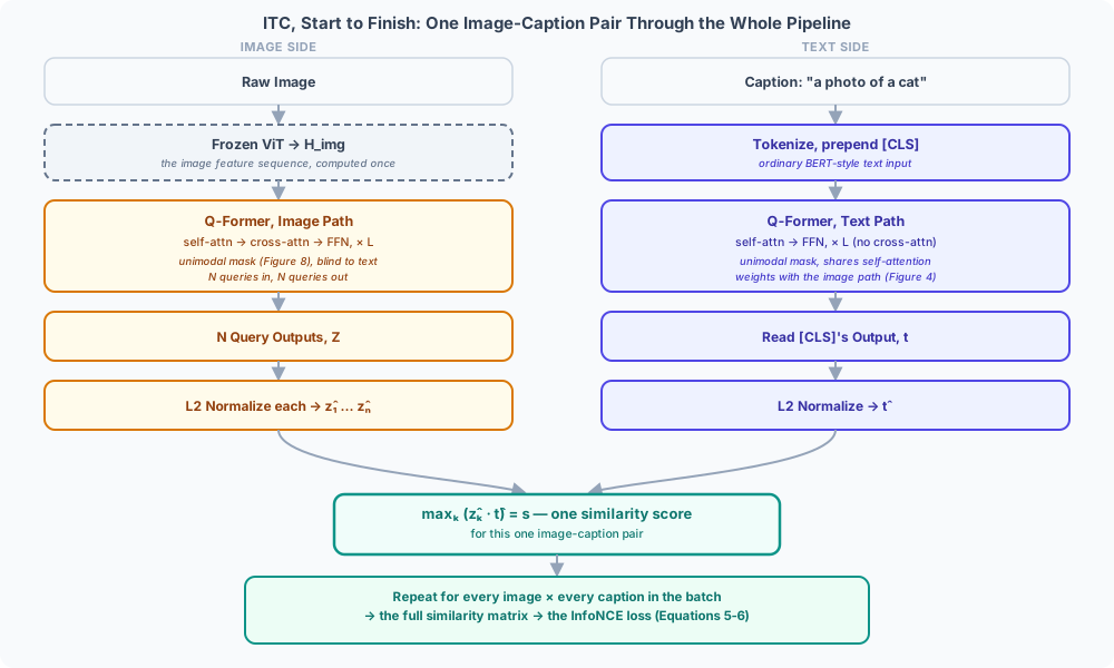
Two things worth fixing in your head before the details: the image side has no [CLS] anywhere — only
query outputs, and it's the maximum similarity across all of them that gets used, Equation (3)
below. The text side does have a real [CLS], prepended the same way BERT's own input
representation does, and that's what gets L2-normalized and compared. The two
vectors that finally meet at the dot product — one query's output, one [CLS] output — are both unit length,
so that dot product is a cosine similarity (bounded between and , largest when the two vectors
point the same way), the identical quantity CLIP's own similarity matrix computes,
not a distance.
3.1. The unimodal mask
ITC's job is to align the queries' representation of an image with a text encoder's representation of a caption — the exact task CLIP's contrastive loss already solves. To keep that comparison honest, the queries and the text aren't allowed to see each other at all while this representation is being built: a unimodal mask blocks every query-to-text and text-to-query attention cell, leaving each side to attend only within itself.
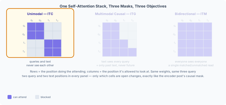
The text side, under this mask, self-attends bidirectionally among its own tokens — standard BERT-style
attention, not CLIP's causally-masked, [EOS]-reading text
tower. That's a direct consequence of the Q-Former's self-attention stack being
initialized from BERT: the text representation used for ITC is read from a prepended [CLS] token, the
same readout position BERT's own classification head uses, not from an appended
[EOS].
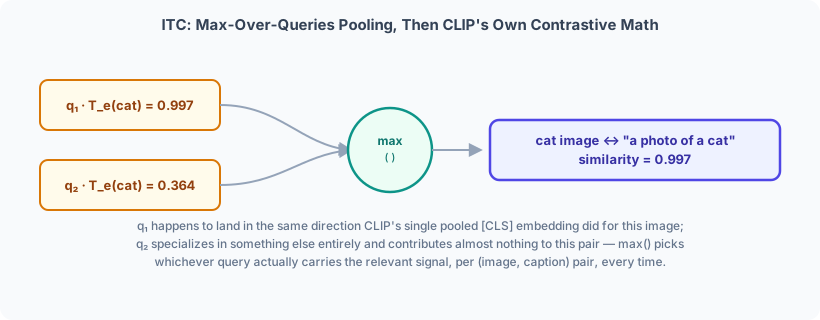
3.2. Max-over-queries pooling
The image side produces separate query output vectors, not one — so there's no single embedding to
compare against the text's [CLS] output the way CLIP compares one against one
. BLIP-2's fix: L2-normalize every query's output and the text's [CLS]
output, exactly CLIP's L2Norm step, then take the maximum similarity across
all queries as the image-text similarity for that pair:
is image 's -th query output, L2-normalized; is caption 's [CLS]
output, L2-normalized. Only the single best-matching query has to carry the signal for any given pair — the
other queries are free to specialize in something else entirely without dragging the similarity score
down.
3.3. Worked example, reusing CLIP's own toy batch
To keep this comparable to CLIP's own worked example directly, reuse its exact
toy batch — four (image, caption) pairs, cat/dog/bird/car — and its exact text embeddings. is
CLIP's own name for them: whatever its text tower produces for a caption, projected and L2-normalized —
Equation (2), the same role plays in Equation (3)
above. Reusing
CLIP's actual numbers here, rather than deriving fresh ones by running a caption through the Q-Former's text
transformer, is purely a narrative shortcut — a stand-in for whatever the Q-Former's own [CLS] output would
look like once normalized, chosen so the numbers stay directly comparable to CLIP's own worked example. For
query 1's output on each image, reuse CLIP's own raw image
vectors, normalized the same way, so lands in the identical direction
CLIP's single pooled embedding did. Query 2 is given a fixed, generic raw vector, [0.5, -0.5, 0.5, -0.5],
the same for every image — a stand-in for a query that happened to specialize in something with no
particular class signal, texture or background detail rather than "what animal is this":
| Image | (query 1, normalized) | (query 2, normalized) |
|---|---|---|
| cat | [0.949, 0.316, 0, 0] | [0.5, -0.5, 0.5, -0.5] |
| dog | [0.316, 0.949, 0, 0] | [0.5, -0.5, 0.5, -0.5] |
| bird | [0, 0, 0.949, 0.316] | [0.5, -0.5, 0.5, -0.5] |
| car | [0, 0, 0.316, 0.949] | [0.5, -0.5, 0.5, -0.5] |
The four values themselves, one row per caption:
| Caption | (text embedding, normalized) |
|---|---|
| "a photo of a cat" | [0.970, 0.243, 0, 0] |
| "a photo of a dog" | [0.243, 0.970, 0, 0] |
| "a photo of a bird" | [0, 0, 0.970, 0.243] |
| "a photo of a car" | [0, 0, 0.243, 0.970] |
Dotting each query against every caption's — worked out one entry at a time for the cat image, whose two normalized queries are and :
| Caption | |||
|---|---|---|---|
| cat | |||
| dog | |||
| bird | |||
| car |
(Every row uses the same two dot products, and — only , the caption's text embedding, changes. 's dot product flips sign between cat/bird and dog/car because its own vector, , has matching-sign components on the cat/bird dimensions and opposite-sign components on the dog/car dimensions — a direct consequence of how it was picked above, not a new computation.) Taking the column-wise maximum gives the cat image's full row:
z1_cat = np.array([0.949, 0.316, 0, 0])
z2_cat = np.array([0.5, -0.5, 0.5, -0.5])
T_e = {
    "cat": np.array([0.970, 0.243, 0, 0]),
    "dog": np.array([0.243, 0.970, 0, 0]),
    "bird": np.array([0, 0, 0.970, 0.243]),
    "car": np.array([0, 0, 0.243, 0.970]),
}

s_cat_image = np.array([max(z1_cat @ T_e[cap], z2_cat @ T_e[cap]) for cap in T_e])
print(np.round(s_cat_image, 3))
# [0.997 0.537 0.364 0.   ]
Against the "cat" caption, scores (identical to CLIP's own cat-image similarity) while only manages — max-pooling correctly keeps 's number. Against "bird," contributes nothing (, since its raw vector has no component on the bird/car dimensions), but 's generic direction happens to overlap that caption's dimensions too, contributing a modest that max-pooling now does pick up — a small amount of unwanted cross-talk from a query that isn't actually tracking anything class-relevant. The diagonal still wins clearly in every row and column, but this is exactly the kind of noise a real 32-query BLIP-2 relies on the sheer number of queries, and a lot more training, to average out.
3.4. The contrastive loss
Once replaces CLIP's , the rest of the loss is unchanged — the identical symmetric InfoNCE shape as Equation (8) through Equation (10), scaled by the same learned temperature :
is the column-wise mirror of Equation (5), exactly the way CLIP's Equation (9) mirrors its own Equation (8). Running the full max-pooled matrix through both directions, at :
T_e = {
    "cat": np.array([0.970, 0.243, 0, 0]),
    "dog": np.array([0.243, 0.970, 0, 0]),
    "bird": np.array([0, 0, 0.970, 0.243]),
    "car": np.array([0, 0, 0.243, 0.970]),
}
q1 = {
    "cat": np.array([0.949, 0.316, 0, 0]),
    "dog": np.array([0.316, 0.949, 0, 0]),
    "bird": np.array([0, 0, 0.949, 0.316]),
    "car": np.array([0, 0, 0.316, 0.949]),
}
q2_generic = np.array([0.5, -0.5, 0.5, -0.5])  # same direction for every image

images = ["cat", "dog", "bird", "car"]
sim_max = np.array([
    [max(q1[img] @ T_e[cap], q2_generic @ T_e[cap]) for cap in images]
    for img in images
])
tau = 10.0
logits = tau * sim_max
row_probs = softmax(logits, axis=1)
col_probs = softmax(logits, axis=0)
L_i2t = -np.mean(np.log(np.diag(row_probs)))
L_t2i = -np.mean(np.log(np.diag(col_probs)))

print(np.round(sim_max, 3))
# [[0.997 0.537 0.364 0.   ]
#  [0.537 0.997 0.364 0.   ]
#  [0.364 0.    0.997 0.537]
#  [0.364 0.    0.537 0.997]]
print(round(L_i2t, 4), round(L_t2i, 4))
# 0.0118 0.0118
— slightly higher than CLIP's own on the identical batch, and the difference is entirely 's generic cross-talk nudging a few off-diagonal logits up. A well-trained Q-Former, with dozens of queries instead of two and real gradient pressure from this exact loss, learns to keep that kind of noise from creeping into the max.
4. Stage 1, Loss 2 — Image-Grounded Text Generation (ITG)
4.1. The multimodal causal mask
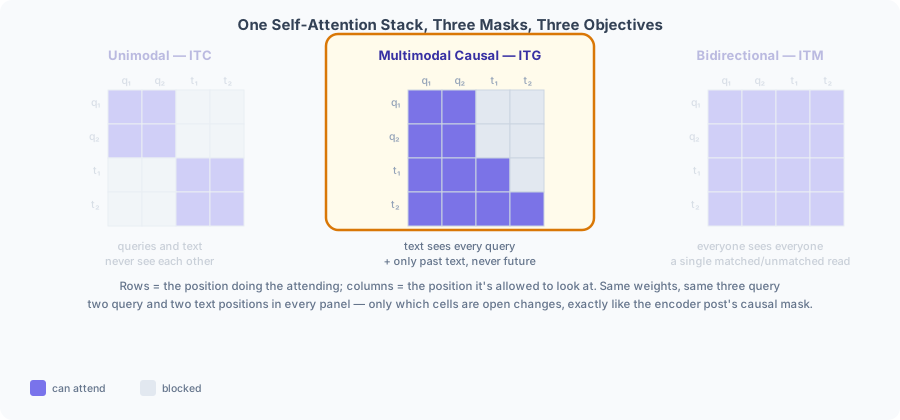
ITG trains the Q-Former to generate a caption directly from the queries, one word at a time — the same next-token objective the decoder post's output layer uses, just grounded in queries instead of a co-trained encoder's output. The mask that makes this work is a hybrid: queries attend to each other bidirectionally, exactly as in ITC; text tokens attend causally to earlier text tokens, the same restriction the encoder post's causal mask enforces for any decoder-style model; and — the one new rule — every text position attends to every query, but no query ever attends to any text token.
4.2. Why this specific asymmetry matters
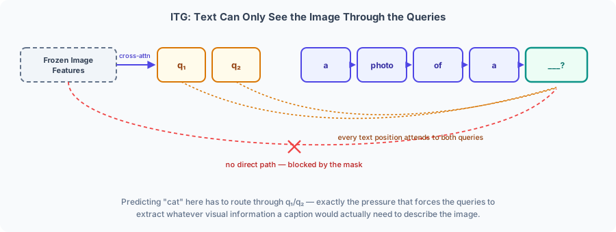
That last rule is the entire point of the objective. Text tokens have no cross-attention layers into the frozen image encoder at all — module 2 already noted this — so the only route from pixels to a generated word runs through the queries. If a query's output doesn't contain whatever visual detail the caption is about to mention, the text transformer has no other way to get it. That's a strictly stronger pressure on the queries than ITC alone provides: ITC only asks a query to be distinguishable from other images' queries; ITG asks the queries, collectively, to contain everything a fluent caption would need to say.
4.3. The generative loss
Structurally the same negative-log-likelihood sum as the decoder post's training objective and BERT's MLM loss, just conditioned on the query outputs instead of an encoder's or a corrupted input:
Each term is the identical linear-projection-plus-softmax shape as the decoder post's output layer, Equation (2):
4.4. Worked example: predicting the last word
Toy generation vocabulary — small enough to fit on screen, big enough to cover a caption:
| Word | a | photo | of | cat | dog | bird | car | <EOS> |
|---|---|---|---|---|---|---|---|---|
| ID | 0 | 1 | 2 | 3 | 4 | 5 | 6 | 7 |
Target caption "a photo of a cat," generated causally: by the time the model is predicting the fifth word, it has already produced "a photo of a" and has both queries to draw on. Running the whole chain isn't repeated here — like BERT's masked-position worked example, this module starts from a clearly-labeled hypothetical for the resulting hidden state:
vocab = ["a", "photo", "of", "cat", "dog", "bird", "car", "<EOS>"]
h_gen = np.array([0.9, 0.3, 0.1, 0.1])

W_vocab = np.array([
    [0.1, 0.1, 0.1, 0.5, -0.2, -0.1, -0.2, -0.1],
    [0.1, 0.2, 0.1, 0.3, 0.1, -0.1, -0.1, -0.2],
    [-0.1, 0.1, 0.2, 0.2, 0.1, 0.1, -0.1, 0.3],
    [0.2, -0.1, 0.1, 0.2, -0.2, 0.1, 0.2, 0.2],
])
b_vocab = np.array([0.1, 0.1, 0.1, 0.1, 0.1, 0.1, 0.1, -0.2])

logits = h_gen @ W_vocab + b_vocab
probs = softmax(logits)
print(vocab[np.argmax(probs)], round(probs.max(), 3))
# cat 0.21
"cat" comes out on top, at — not overwhelmingly confident, since and here are hand-picked stand-ins rather than the product of real training, but enough to show the mechanism correctly favoring the right word once the queries actually carry cat-relevant information.
5. Stage 1, Loss 3 — Image-Text Matching (ITM)
5.1. The bidirectional mask
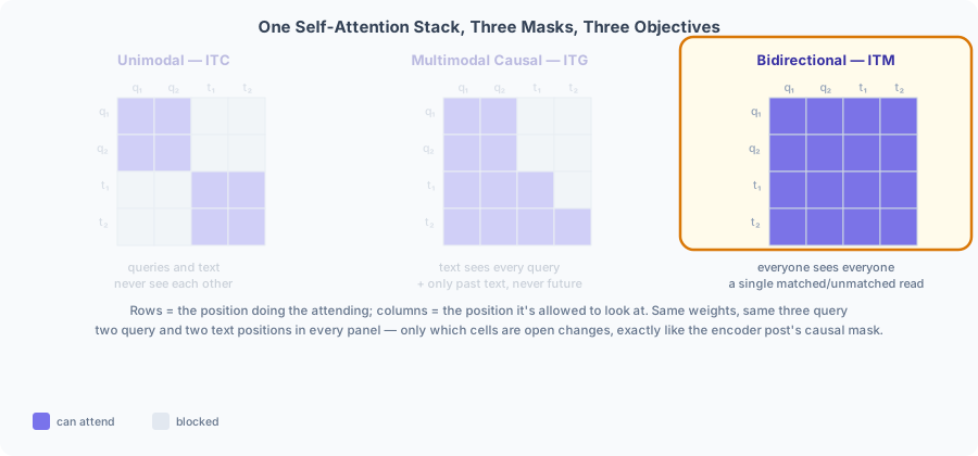
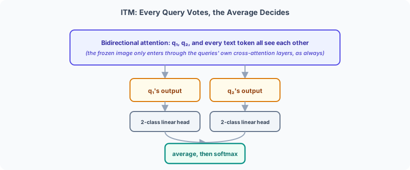
ITM asks the simplest question of the three: does this image and this caption actually belong together, yes or no? Since there's no generation step and no risk of "reading the answer off the input" the way bidirectional pretraining without corruption would for BERT — the label here is external (a real pair vs. a swapped-in mismatched one), not something sitting inside the sequence itself — ITM opens the mask completely: queries and text attend to each other freely, in both directions.
5.2. Averaging over queries
Every query's final output, under this fully open mask, is now a genuinely multimodal representation —
it's had direct access to the text as well as the frozen image. Each of the query outputs is scored
independently by the same small 2-class linear head (match / no-match), and the logits are averaged
across queries before the softmax, rather than reading a single [CLS]-style position the way BERT's
NSP head does:
Note: the real BLIP-2 paper also borrows a hard negative mining strategy from ALBEF [6] for this objective — rather than pairing every image with a uniformly random mismatched caption, negatives are sampled with probability proportional to how similar they already look under the ITC similarity scores just computed. A random mismatch (a cat photo against "a photo of a car") is trivial for the classifier to reject; a near-mismatch, sampled specifically because ITC already ranked it deceptively close, is what actually teaches the head something.
5.3. Worked example
Hypothetical final hidden states for the two queries, cat image paired with its own matching caption — the positive-pair case:
h1 = np.array([0.6, 0.5, 0.2, 0.1])
h2 = np.array([0.4, 0.6, 0.1, 0.3])

W_itm = np.array([[0.5, -0.3], [-0.2, 0.4], [0.3, -0.1], [-0.4, 0.6]])
b_itm = np.array([0.0, 0.0])

logits1 = h1 @ W_itm + b_itm
logits2 = h2 @ W_itm + b_itm
avg_logits = (logits1 + logits2) / 2
probs = softmax(avg_logits)
print(np.round(probs, 3))
# [0.483 0.518]
Close to a coin flip, the same story as BERT's own NSP worked example — untrained, hand-picked has no particular reason to be confident. What the mechanism demonstrates is the averaging itself: query 1 leans slightly toward "match" ( as raw logits), query 2 leans slightly the other way (), and the final decision is neither query's alone.
6. One Shared Stack, Three Masks
6.1. Why this can't be one forward pass
BERT's MLM and NSP heads share a single forward pass — both read from the same bidirectional encoder output, computed once, because both tasks are happy with the identical, fully-open mask. ITC, ITG, and ITM aren't compatible that way. ITC's unimodal mask requires queries and text to be mutually invisible; ITM's bidirectional mask requires the opposite. No single mask can satisfy both at once, so — unlike BERT — a BLIP-2 training step runs the shared self-attention stack three separate times per batch, once under each mask (Figure 3's three mask panels on the right, or Figures 8/10/12 for each one in detail), and sums the three resulting losses. All three run every step, on every batch — not one objective at a time, not alternating, not curriculum-scheduled:
Every one of those three passes updates the same underlying weights — the queries, the shared self-attention layers, the cross-attention layers, all of it — so nothing about the Q-Former's parameters is task-specific the way BERT's separate MLM and NSP heads are. What's task-specific is purely which mask gets applied on a given forward pass, the identical "one mechanism, several masking patterns" idea UniLM [7] introduced for unifying encoder- and decoder-style pretraining in a single model, applied here across three objectives instead of two.
6.2. Where the mask actually enters the computation
To be unambiguous about what "pass" means here: it's neither alternating batches (batch 1 trains ITC, batch 2 trains ITG, ...) nor splitting one batch by task (some images in the batch go through ITC, others through ITM). Every image-caption pair in every batch goes through all three passes, every single step. The three passes happen back to back within one training step, on the same batch, and only then does a single combined loss get backpropagated:
for batch in dataloader:
    queries = learned_query_embeddings         # same for the whole batch
    text = tokenize(batch.captions)
    H_img = frozen_vit(batch.images)            # computed once, reused by every pass's cross-attention

    hidden_itc = self_attention(queries, text, mask=M_unimodal)          # pass 1
    hidden_itg = self_attention(queries, text, mask=M_multimodal_causal) # pass 2
    hidden_itm = self_attention(queries, text, mask=M_bidirectional)     # pass 3, M is all zeros

    loss = itc_loss(hidden_itc) + itg_loss(hidden_itg) + itm_loss(hidden_itm)
    loss.backward()   # one backward pass, gradients from all three flow into the same shared weights
    optimizer.step()  # one weight update per batch, not three
Same function, same weights inside it, called three times per batch with three different masks — so
hidden_itc, hidden_itg, and hidden_itm are three genuinely different sets of numbers, computed
independently. ITC's loss reads only from hidden_itc; ITG's only from hidden_itg; ITM's only from
hidden_itm. Each mask belongs to exactly one pass and exactly one loss — there's no sharing of a single
pass's output between objectives, and no batch or example ever skips one of the three.
The mask itself, inside each of those three calls, is the same additive-bias mechanism the encoder post's causal mask uses:
is an matrix of s (visible) and s (blocked), where queries occupy
positions and text occupies . M_unimodal zeroes out the entire query-text and
text-query blocks; M_bidirectional is all zeros; M_multimodal_causal keeps the query block open, adds a
causal triangle inside the text block, and opens text-to-query while leaving query-to-text blocked.
Cross-attention never sees any of these three masks — it isn't masked in any of the three passes. It's always the same computation: queries (only) attending to the full, unmasked , exactly as module 2 described. Text has no cross-attention layers to begin with, so there's nothing there to mask either. The three-mask story is entirely a self-attention story, and it plays out as three independent executions of it, not one.
7. Stage 2 — Bridging to a Frozen LLM
7.1. Still training — a second phase, not deployment
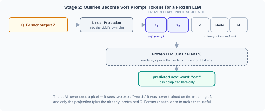
Stage 2 is a second, separate training phase, not the point where a finished Q-Former gets deployed and used. The Q-Former doesn't stop learning at the end of stage 1 — it keeps training, starting from its stage-1 weights rather than frozen there, and a brand-new linear projection layer trains from scratch alongside it. What's new in stage 2 is only the source of gradient: instead of ITC, ITG, and ITM, the signal now comes from the frozen LLM's own generative loss. Actual use of the finished system — a new image in, an answer out, no gradients anywhere — only happens once both stages are behind it.
7.2. What stage 1 already bought
By the end of stage 1, the queries have been pushed by three different pressures at once, every step, summed together: ITC makes them discriminative against other images' queries; ITG makes them collectively sufficient to generate a fluent caption; ITM makes them sensitive to whether a specific caption actually matches. None of that required the expensive frozen LLM even once. Stage 2's job is comparatively small by comparison: take queries that are already this well-organized, and teach one linear layer to hand them to a language model that has never seen one before.
7.3. The projection
Structurally the simplest step in the whole pipeline — one more linear layer, the same shape of computation as every projection already used in this series, mapping the Q-Former's own dimension into whatever dimension the frozen LLM's own token embeddings live in:
Reusing module 2's own worked cross-attention output, Equation (2), as :
query_repr = np.array([
    [0.548, 0.804, 0.548, 0.804],
    [0.542, 0.790, 0.542, 0.790],
])
W_proj = np.array([
    [0.6, 0.1, -0.1, 0.2],
    [0.1, 0.5, 0.2, -0.1],
    [-0.1, 0.2, 0.6, 0.1],
    [0.2, -0.1, 0.1, 0.5],
])
b_proj = np.array([0.05, 0.05, 0.05, 0.05])

soft_prompt = query_repr @ W_proj + b_proj
print(np.round(soft_prompt, 3))
# [[0.565 0.536 0.565 0.536]
#  [0.558 0.529 0.558 0.529]]
7.4. Soft prompts, and the generative loss
and get prepended directly in front of the caption's ordinary tokenized text embeddings, as if they were two more words in the sequence — "soft" because, unlike every other token the LLM has ever seen, these two were never looked up from a fixed embedding table; they're continuous vectors the projection produced on the fly. The frozen LLM then runs its own unmodified forward pass over , and the loss is computed only over the text portion — the identical next-token shape as Equation (7) above, now with the frozen LLM's own (much larger) vocabulary and output layer in place of the Q-Former's:
vocab = ["a", "photo", "of", "cat", "dog", "bird", "car", "<EOS>"]
h_gen2 = np.array([0.85, 0.35, 0.15, 0.05])

W_vocab_llm = np.array([
    [0.15, 0.1, 0.1, 0.45, -0.1, -0.2, -0.1, -0.1],
    [0.1, 0.2, 0.15, 0.35, 0.05, -0.1, -0.15, -0.1],
    [-0.1, 0.1, 0.2, 0.25, 0.1, 0.1, -0.1, 0.2],
    [0.2, -0.1, 0.1, 0.3, -0.15, 0.1, 0.15, 0.1],
])
b_vocab_llm = np.array([0.1, 0.1, 0.1, 0.15, 0.1, 0.1, 0.1, -0.2])

logits = h_gen2 @ W_vocab_llm + b_vocab_llm
probs = softmax(logits)
print(vocab[np.argmax(probs)], round(probs.max(), 3))
# cat 0.211
Nearly identical numbers to Equation (9)'s ITG result, and deliberately so — this is the same next-token mechanism, with a different (frozen, much larger) model reading the queries this time.
7.5. Two flavors of frozen LLM
BLIP-2 pairs the Q-Former with two different kinds of frozen LLM, and the loss shape above is really a simplification of the decoder-only case. With a decoder-only LLM like OPT [8], the whole target text is generated causally after the soft prompt, exactly as worked out above. With an encoder-decoder LLM like FlanT5 [9], the target text is split into a prefix (concatenated with the soft prompt and fed to the encoder side) and a suffix (the decoder's actual generation target) — a prefix language modeling setup, structurally the original Transformer's encoder-decoder split rather than a pure decoder stack. Either way, the LLM's own weights never move; only the Q-Former (continuing to train from its stage-1 state) and the newly added projection layer receive gradient.
8. What BLIP-2 Buys You
8.1. Trainable parameters, in perspective
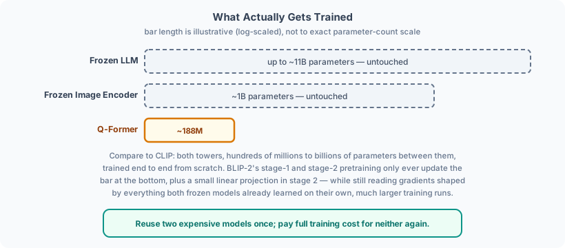
The real Q-Former is around 188M parameters — a fraction of either the frozen image encoder or the frozen LLM it sits between, both of which stay entirely untouched across both pretraining stages. CLIP, by contrast, trains both of its towers, hundreds of millions to billions of parameters between them, end to end from nothing. BLIP-2's whole pitch is that reusing two already-paid-for training runs, and training only a small bridge between them, gets you a usable vision-language system for a fraction of that cost — provided the bridge has enough capacity, and is pretrained against the right cheap objectives first, to actually close the modality gap module 1 opened with.
8.2. Where this leads
Every mechanism in this post is something this series had already built before BLIP-2: BERT's self-attention as the Q-Former's initialization, the decoder's cross-attention reaching into a frozen rather than co-trained source, CLIP's contrastive loss reused almost unchanged for ITC, and the decoder's own next-token loss for both ITG and stage 2's generative objective. What BLIP-2 adds is the combination: one small module, three masks over one shared stack, and a soft-prompt bridge into a model that never has to be retrained. InstructBLIP [10] pushes the same recipe further with instruction tuning; a later line of work asks whether the Q-Former's three-objective pretraining is even necessary at all, or whether a single trained linear layer plus instruction-tuned data can do the same job — which is exactly where LLaVA picks up.
9. Putting It All Together
9.1. Scope: what's novel here, and what's assumed
Everything below is BLIP-2-specific: the Q-Former block, the three masks, the three losses, and the two
training steps. Standard building blocks this series already covered elsewhere — masked self-attention,
cross-attention, a feed-forward network, softmax, tokenization, and the frozen ViT and frozen LLM themselves
— are left as stubs with a docstring pointing at where they actually get built. This is architecture-level
reference code: it shows the real data flow and the real shapes, but frozen_vit and frozen_llm_generate
are undefined, so unlike the toy snippets earlier in this post, it isn't something you can paste and run.
import numpy as np

def self_attention(x, Wq, Wk, Wv, mask=None):
    """softmax(QK^T / sqrt(d_k) + M) V. Same function as the encoder post's
    MaskedAttention — Q, K, V all come from the same input x."""
    Q, K, V = x @ Wq, x @ Wk, x @ Wv
    scores = Q @ K.T / np.sqrt(K.shape[-1])
    if mask is not None:
        scores = scores + mask
    return softmax(scores, axis=-1) @ V

def cross_attention(query_x, source, Wq, Wk, Wv):
    """Q from query_x, K/V from a different sequence, unmasked — the decoder
    post's cross-attention block."""
    Q, K, V = query_x @ Wq, source @ Wk, source @ Wv
    scores = Q @ K.T / np.sqrt(K.shape[-1])
    return softmax(scores, axis=-1) @ V

def feed_forward(x, W1, b1, W2, b2):
    return np.maximum(0, x @ W1 + b1) @ W2 + b2

def softmax(x, axis=-1):
    e = np.exp(x - np.max(x, axis=axis, keepdims=True))
    return e / np.sum(e, axis=axis, keepdims=True)

def linear(x, W, b):
    return x @ W + b

def frozen_vit(images):
    """Frozen throughout both stages — module 1's whole point. Returns H_img,
    the patch feature sequence."""
    ...

def frozen_llm_generate(soft_prompt, captions):
    """Frozen decoder-only LLM. Prefixes soft_prompt to the tokenized caption
    and returns the teacher-forced generation loss — module 7. Never updated."""
    ...

def tokenize(captions):
    ...
9.2. The three attention masks
The one piece of state that actually changes between ITC, ITG, and ITM — module 6's additive-bias mask, built once per pass:
def build_mask(kind, N, T):
    """(N+T) x (N+T) additive mask. Queries occupy rows/cols [0, N); text
    occupies [N, N+T). 0 = visible, -inf = blocked."""
    M = np.zeros((N + T, N + T))
    if kind == "unimodal":                 # ITC — module 3
        M[:N, N:] = -np.inf
        M[N:, :N] = -np.inf
    elif kind == "bidirectional":          # ITM — module 5, already fully open
        pass
    elif kind == "multimodal_causal":      # ITG — module 4
        M[:N, N:] = -np.inf                                    # queries can't see text
        M[N:, N:] = np.triu(np.full((T, T), -np.inf), k=1)     # text: causal, among itself
        # M[N:, :N] stays 0 — every text position sees every query
    return M
9.3. One Q-Former block, and the full stack
Shared self-attention, then cross-attention on the image row only, then two separate feed-forward networks — Figures 4-6's block shape, with cross-attention alternating every other block:
def qformer_block(q_hidden, t_hidden, H_img, mask, w, has_cross_attention):
    """`w` holds this block's own weights — its self-attention Wq/Wk/Wv, its own
    cross-attention Wq/Wk/Wv (if it has one), and its own two FFNs. Nothing here
    is reused from any other block or any other pass (equation 1)."""
    combined = q_hidden if t_hidden is None else np.concatenate([q_hidden, t_hidden], axis=0)
    attn_out = self_attention(combined, w.Wq_self, w.Wk_self, w.Wv_self, mask=mask)
    N = len(q_hidden)
    q_hidden, t_hidden = attn_out[:N], (None if t_hidden is None else attn_out[N:])

    if has_cross_attention:
        q_hidden = q_hidden + cross_attention(q_hidden, H_img, w.Wq_cross, w.Wk_cross, w.Wv_cross)
        # text never gets a cross-attention call — module 2's whole point

    q_hidden = feed_forward(q_hidden, *w.ffn_query)
    t_hidden = None if t_hidden is None else feed_forward(t_hidden, *w.ffn_text)
    return q_hidden, t_hidden

def qformer_stack(queries, text, H_img, mask, layers):
    """L blocks, cross-attention alternating every other block (Figure 5)."""
    q_hidden, t_hidden = queries, text
    for i, w in enumerate(layers):
        has_cross = (i % 2 == 0)   # block 1, 3, 5, ... in Figure 5's 1-indexed labeling
        q_hidden, t_hidden = qformer_block(q_hidden, t_hidden, H_img, mask, w, has_cross)
    return q_hidden, t_hidden   # Z, and the final text hidden states
9.4. The three stage-1 losses
Each one reads from exactly one of the three passes — module 6 already covered why none of them can be shared:
def itc_loss(Z_batch, t_batch, temperature):
    """Z_batch: one (N, d) query-output array per image. t_batch: one (d,)
    text [CLS] output per caption. Max-over-queries similarity (equation 3),
    then CLIP's own contrastive loss (equations 5, 6)."""
    B = len(Z_batch)
    Z_hat = [z / np.linalg.norm(z, axis=-1, keepdims=True) for z in Z_batch]
    t_hat = [t / np.linalg.norm(t) for t in t_batch]
    sim = np.array([[np.max(Z_hat[i] @ t_hat[j]) for j in range(B)] for i in range(B)])
    logits = temperature * sim
    i2t = -np.mean(np.log(softmax(logits, axis=1)[np.arange(B), np.arange(B)]))
    t2i = -np.mean(np.log(softmax(logits.T, axis=1)[np.arange(B), np.arange(B)]))
    return 0.5 * (i2t + t2i)

def itg_loss(t_hidden, target_ids, W_vocab, b_vocab):
    """Reads only the text row (equations 7, 8) — Z never enters this formula
    directly; its influence already reached t_hidden through the multimodal
    causal mask's self-attention."""
    probs = softmax(linear(t_hidden, W_vocab, b_vocab), axis=-1)
    return -np.mean([np.log(probs[i, target_ids[i]]) for i in range(len(target_ids))])

def itm_loss(Z, label, W_itm, b_itm):
    """Per-query 2-class head, averaged before the softmax (equation 10)."""
    avg_logits = np.mean([linear(z, W_itm, b_itm) for z in Z], axis=0)
    return -np.log(softmax(avg_logits)[label])
9.5. Stage 1: one training step
Three full passes on the same batch, one combined loss, one weight update — the loop this section has been building up to since module 6:
def stage1_step(batch, layers, learned_queries, heads):
    N = len(learned_queries)
    H_img = frozen_vit(batch.images)          # run once, shared by all three passes' cross-attention
    text = tokenize(batch.captions)
    T = text.shape[1]

    Z_itc, t_itc = qformer_stack(learned_queries, text, H_img, build_mask("unimodal", N, T), layers)
    Z_itg, t_itg = qformer_stack(learned_queries, text, H_img, build_mask("multimodal_causal", N, T), layers)
    Z_itm, t_itm = qformer_stack(learned_queries, text, H_img, build_mask("bidirectional", N, T), layers)

    loss = (
        itc_loss(Z_itc, t_itc[:, 0], heads.temperature)
        + itg_loss(t_itg, batch.next_token_ids, *heads.vocab_proj)
        + itm_loss(Z_itm, batch.match_labels, *heads.itm_head)
    )
    loss.backward()   # gradients from all three passes land on the same shared `layers`
    optimizer.step()  # one update per batch, not three
9.6. Stage 2: bridging to the frozen LLM
Only the queries go through the Q-Former here — no text row, so no mask to choose either (module 7):
def stage2_step(batch, layers, learned_queries, W_proj, b_proj):
    H_img = frozen_vit(batch.images)
    Z, _ = qformer_stack(learned_queries, text=None, H_img=H_img, mask=None, layers=layers)

    soft_prompt = linear(Z, W_proj, b_proj)                  # equation 12
    loss = frozen_llm_generate(soft_prompt, batch.captions)  # equation 14, teacher-forced

    loss.backward()   # reaches W_proj and layers; the frozen LLM gets no gradient at all
    optimizer.step()
That's the entire system: one qformer_block, reused for every block of every pass of both stages; one
build_mask, reused for all three stage-1 objectives; and everything this post derived by hand along the way
— equations 1 through 15 — is exactly the math running inside these dozen functions.
References
- [1]Li, Li, Savarese & Hoi (2023). BLIP-2: Bootstrapping Language-Image Pre-training with Frozen Image Encoders and Large Language Models. International Conference on Machine Learning (ICML).
- [2]Li, Li, Xiong & Hoi (2022). BLIP: Bootstrapping Language-Image Pre-training for Unified Vision-Language Understanding and Generation. International Conference on Machine Learning (ICML).
- [3]Devlin, Chang, Lee & Toutanova (2018). BERT: Pre-training of Deep Bidirectional Transformers for Language Understanding. North American Chapter of the Association for Computational Linguistics (NAACL).
- [4]Dosovitskiy et al. (2020). An Image is Worth 16x16 Words: Transformers for Image Recognition at Scale. International Conference on Learning Representations (ICLR).
- [5]Radford et al. (2021). Learning Transferable Visual Models From Natural Language Supervision. International Conference on Machine Learning (ICML).
- [6]Li, Selvaraju, Gotmare, Joty, Xiong & Hoi (2021). Align before Fuse: Vision and Language Representation Learning with Momentum Distillation (ALBEF). Neural Information Processing Systems (NeurIPS).
- [7]Dong et al. (2019). Unified Language Model Pre-training for Natural Language Understanding and Generation (UniLM). Neural Information Processing Systems (NeurIPS).
- [8]Zhang et al. (2022). OPT: Open Pre-trained Transformer Language Models.
- [9]Chung et al. (2022). Scaling Instruction-Finetuned Language Models (Flan-T5).
- [10]Dai et al. (2023). InstructBLIP: Towards General-purpose Vision-Language Models with Instruction Tuning. Neural Information Processing Systems (NeurIPS).