Every model in this series so far has been trained against a fixed, closed vocabulary of answers.
The decoder post predicts the next word from a fixed
vocabulary of tokens. BERT's fine-tuning module predicts one of classes,
where is chosen and frozen into a weight matrix's shape before training even starts. ViT's
classification head does the same for images: three toy classes, cat, dog,
bird, baked into 's three output columns. Every one of those models has to be retrained, or at least
have a new head fine-tuned, the moment you want to recognize a class nobody trained it on.
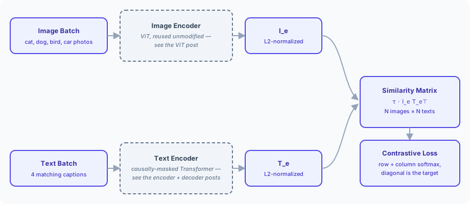
CLIP [1] sidesteps that entirely, and does it with a genuinely different pretraining objective, not a bigger version of the same one. Instead of predicting a class label, CLIP is trained to decide whether an image and a caption belong together — pulling the embeddings of matching pairs close together and pushing mismatched pairs apart, across hundreds of millions of (image, caption) pairs scraped from the internet, with no hand-labeled class at all. The training signal is just whatever a real caption already says about a real image. Once that joint embedding space exists, "classification" for any set of classes at all — including ones CLIP never saw a single labeled example of — falls out for free: describe each class in a sentence, embed the sentences, and see which one the image's embedding sits closest to.
This post assumes you've read the ViT post and the encoder / decoder posts — CLIP's two towers are exactly those architectures, reused unmodified, and none of their internals are re-derived here. What's new is everything about how the two towers are trained together: projecting both into one shared space, the contrastive loss that shapes that space, and the zero-shot classification trick it unlocks.
Contents
- Two Towers, One Embedding Space — reusing ViT's image encoder and a causally-masked Transformer text encoder, projected and L2-normalized into a shared embedding space
- The Similarity Matrix — cosine similarity between every image and every caption in a batch, scaled by a learned temperature
- The Contrastive Loss (InfoNCE) — symmetric cross-entropy across the rows and columns of that matrix
- Zero-Shot Classification — reusing the exact same computation at inference time, with no classification head at all
1. Two Towers, One Embedding Space
1.1. Two independent encoders
CLIP is two separate models trained jointly, not one model with two input types mixed together. An image encoder turns an image into a vector; a text encoder turns a caption into a vector; the two never attend to each other, never share weights, and never see each other's input directly — the only thing that ties them together is the loss function, covered in the Contrastive Loss module below.
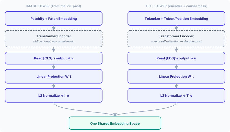
The image encoder is ViT, completely unmodified: patchify, linearly project,
prepend [CLS], add learnable positional embeddings, run through the Transformer encoder, and read
[CLS]'s final output. Nothing about that pipeline changes here — the original CLIP paper also offers a
ResNet variant [1], but the ViT variant is the one that lines up with this series, so
that's what's used below.
The text encoder is a Transformer encoder with one specific change: causal masking, the same mechanism the decoder post's Self-Attention module introduced — Equation (8) and Equation (9) — applied on its own, with no cross-attention and no separate decoder stack. That's a genuine departure from every text encoder used earlier in this series: the encoder post and BERT are both fully bidirectional, every position seeing every other position. CLIP's text tower can't do that — token 's final representation is only ever built from tokens , exactly the decoder post's guarantee. CLIP's paper motivates this choice by compatibility: a causally-masked text encoder can be initialized from, or later extended into, a real language model, an option a bidirectional encoder forecloses [1].
Note: causal masking is also why CLIP reads the text encoder's output from a different position than BERT and ViT read theirs.
[CLS]sits at the front of BERT's and ViT's sequences precisely because those encoders are bidirectional — every position,[CLS]included, can see the entire sequence, so where you place the read-out token doesn't matter for how much context it has access to. That's not true here: with causal masking, only the last position has attended to every earlier token; the first position has attended to nothing but itself. So CLIP appends a special[EOS]token to the end of the sequence instead, and reads its output — the one position guaranteed to have seen the whole caption.
1.2. What "appending EOS" actually means
To make that concrete: [EOS] is a real, literal extra token, added to the tokenized caption exactly the
way [CLS] and [SEP] were literal extra tokens in BERT's Input Representation
module — it gets its own row in the token embedding table, its own position in
the sequence, and its own position embedding, just like every other token. It isn't a name for "the last
word" or a flag set on an existing token; it's appended after the caption's own tokens, so it's always the
very last position in the sequence, whatever the caption's length happens to be. For the caption "a photo
of a cat," using this series' own whole-word tokenization, the sequence the text encoder actually receives
is six tokens long:
| Position | 0 | 1 | 2 | 3 | 4 | 5 |
|---|---|---|---|---|---|---|
| Token | a | photo | of | a | cat | [EOS] |
Causal masking — Equation (8) and Equation (9) — means position 's
self-attention can only look at positions . Position 0 ("a") can only see itself. Position 5
([EOS]), being last, is the only position whose attention is unrestricted across the whole sequence —
it can see all six tokens, because none of them are in its future. That's the entire reason [EOS] is
placed at the end rather than the start: a token's position determines how much of the sequence it's
allowed to attend to under a causal mask, and only one position — the last one — is allowed to see
everything.
![Diagram of a 6-token caption with a causal mask showing only [EOS] attends to every position](/images/understanding-clip/text-tower-eos-readout.svg)
Running this six-token sequence through the causally-masked encoder stack produces six output vectors, one
per position — but only , [EOS]'s own output, is read out as in Equation (1) below. The
other five did real work getting there (every later position's self-attention pulled information from every
earlier one, including them), but nothing downstream consumes their vectors directly — the identical "every
position computes something, only one position gets read" pattern BERT's [CLS]
and ViT's [CLS] already used, just with the readout token moved from the front
of the sequence to the back.
Note: real CLIP also prepends a
[SOS]("start of sequence") token before the caption's own tokens, so the true sequence is[SOS] a photo of a cat [EOS][1]. It's omitted from the table above because it doesn't change anything about this explanation — under a causal mask, whatever sits in position 0 can only ever attend to itself, whether that position holds "a" or[SOS]. It matters for other reasons (a consistent starting point for every sequence, and compatibility with autoregressive language-model training, the same motivation given for causal masking itself above) but not for why[EOS]specifically is what gets read out.
1.3. Projecting into a shared space
and don't have to produce vectors of the same size — ViT's embedding dimension and the text encoder's embedding dimension are independent architectural choices, and in general they're different. So before the two towers' outputs can be compared at all, each is passed through its own separate learned linear projection into one common dimension, then L2-normalized to unit length:
is ViT's [CLS] output, exactly the classification head module's; is the text encoder's [EOS] output. is , is
— two independent weight matrices, learned during training, mapping each tower's own
native dimension into the one shared dimension . divides a vector by its own length:
Every and every this pipeline ever produces has length exactly 1, by construction. That's not a detail to skip past — the entire next module depends on it.
1.4. The toy batch
Four (image, caption) pairs, small enough to work through by hand — the same cat / dog / bird classes
the ViT post's classification head used, plus car as a fourth, clearly
unrelated class:
| # | Image | Caption |
|---|---|---|
| 1 | cat photo | "a photo of a cat" |
| 2 | dog photo | "a photo of a dog" |
| 3 | bird photo | "a photo of a bird" |
| 4 | car photo | "a photo of a car" |
Running each image through and , and each caption through and , isn't repeated here — it's exactly the ViT and encoder/decoder machinery from the linked posts, unmodified. So, like the ViT post's classification head and BERT's pretraining heads before it, this module starts from a clearly-labeled hypothetical: suppose and come out as
| Image | (raw) |
|---|---|
| cat | [3, 1, 0, 0] |
| dog | [1, 3, 0, 0] |
| bird | [0, 0, 3, 1] |
| car | [0, 0, 1, 3] |
| Caption | (raw) |
|---|---|
| "a photo of a cat" | [4, 1, 0, 0] |
| "a photo of a dog" | [1, 4, 0, 0] |
| "a photo of a bird" | [0, 0, 4, 1] |
| "a photo of a car" | [0, 0, 1, 4] |
Note: unlike the hypothetical outputs earlier posts used — ViT's and BERT's and , both picked to sit near untrained, close-to-chance territory — the numbers above are picked to already look like what a trained CLIP would output: each image's vector overlaps heavily with its own caption's vector and not with the others'. That's deliberate. The point of this post's remaining sections is to show what a good joint embedding space does, not to re-derive near-random arithmetic a fifth time.
Worked example for the cat image, whose raw vector is [3, 1, 0, 0] — norm :
Every raw image vector above has norm and every raw caption vector has norm — chosen that way purely to keep the arithmetic uniform across the batch. Applying Equation (4)'s division to all eight vectors:
| dim 1 | dim 2 | dim 3 | dim 4 | |
|---|---|---|---|---|
| : cat | 0.949 | 0.316 | 0 | 0 |
| : dog | 0.316 | 0.949 | 0 | 0 |
| : bird | 0 | 0 | 0.949 | 0.316 |
| : car | 0 | 0 | 0.316 | 0.949 |
| : "cat" | 0.970 | 0.243 | 0 | 0 |
| : "dog" | 0.243 | 0.970 | 0 | 0 |
| : "bird" | 0 | 0 | 0.970 | 0.243 |
| : "car" | 0 | 0 | 0.243 | 0.970 |
import numpy as np

image_raw = {
    "cat": np.array([3, 1, 0, 0], dtype=float),
    "dog": np.array([1, 3, 0, 0], dtype=float),
    "bird": np.array([0, 0, 3, 1], dtype=float),
    "car": np.array([0, 0, 1, 3], dtype=float),
}
text_raw = {
    "cat": np.array([4, 1, 0, 0], dtype=float),
    "dog": np.array([1, 4, 0, 0], dtype=float),
    "bird": np.array([0, 0, 4, 1], dtype=float),
    "car": np.array([0, 0, 1, 4], dtype=float),
}

def l2norm(x):
    return x / np.linalg.norm(x)

I_e = {k: l2norm(v) for k, v in image_raw.items()}
T_e = {k: l2norm(v) for k, v in text_raw.items()}
print(np.round(I_e["cat"], 3))
# [0.949 0.316 0.    0.   ]
print(np.round(T_e["cat"], 3))
# [0.970 0.243 0.    0.   ]
Notice the structure this particular choice of numbers produces: cat and dog share components on
dimensions 1-2, bird and car share components on dimensions 3-4, and the two groups are completely
orthogonal to each other. That's purely a property of these hand-picked toy vectors, not a claim about real
semantic relationships between the four classes — it's what makes the next module's arithmetic land on
clean numbers.
2. The Similarity Matrix
2.1. Cosine similarity, for free
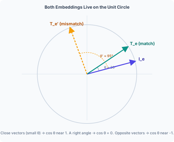
Because every and is unit length — the whole reason for Equation (3) — their dot product isn't just "some number." It's exactly the cosine of the angle between them:
since both norms on the right are 1. This is the reason L2-normalizing is worth a whole equation of its own rather than being an implementation detail: it turns the general dot product — unbounded, and sensitive to each vector's length as well as its direction — into a single number between and that only depends on direction. Two embeddings pointing the same way score 1 regardless of how long the raw projections happened to be; two at right angles score 0; two pointing opposite ways score .
2.2. Scaling by a learned temperature
Cosine similarity alone is a fairly narrow, gently-sloped signal — even a strongly matched pair rarely gets much above 0.3-0.4 in a real trained model. Softmax over a narrow range of logits produces a soft, unconfident distribution, so CLIP scales every similarity by a learned scalar before the softmax ever sees it:
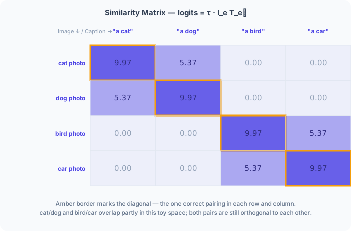
is an matrix — images by captions, one batch's worth — whose entry is , exactly Equation (5)'s cosine similarity between image and caption . is parameterized as , with the actual learned parameter, purely so is guaranteed positive no matter what value takes — an unconstrained scalar is easier to optimize with gradient descent than one with a hard positivity constraint bolted on. Real CLIP initializes so that , following prior contrastive work [6], and clips to never exceed 100 during training, to keep the softmax below from saturating into numerical instability. This worked example uses — close to that real initial value, chosen mainly to keep the hand arithmetic round.
Worked example for the cat image's row — its cosine similarities to all four captions, computed by taking the dot product of the cat row of against every row of , then multiplying by :
(The first entry: , times , gives , rounded to . The second entry follows the same dot product against the "dog" caption's row; the last two are 0 because the cat image vector has nothing but zeros in dimensions 3 and 4, exactly where the bird and car captions carry all their weight.)
2.3. The full matrix
The same computation, all 16 pairs:
tau = 10.0
images = ["cat", "dog", "bird", "car"]
captions = ["cat", "dog", "bird", "car"]

I_mat = np.array([I_e[k] for k in images])
T_mat = np.array([T_e[k] for k in captions])

logits = tau * (I_mat @ T_mat.T)
print(np.round(logits, 2))
# [[9.97 5.37 0.   0.  ]
#  [5.37 9.97 0.   0.  ]
#  [0.   0.   9.97 5.37]
#  [0.   0.   5.37 9.97]]
Every diagonal entry — image against its own caption — is the largest value in both its row and its column. That's exactly what a well-trained joint embedding space should produce, and it's the property the next module's loss function is built to reward.
3. The Contrastive Loss (InfoNCE)
3.1. An -way classification problem, twice
Look at the cat image's row from Equation (7) again: four numbers, one per caption in the batch. That's structurally identical to every classification logit vector this series has produced — Equation (8)'s masked-word logits, Equation (5)'s class logits — just with the "classes" being this batch's four captions instead of a fixed vocabulary. Softmax turns that row into a probability distribution over "which caption in the batch matches this image," and the correct answer is always whichever caption came paired with it — the diagonal entry.
The same argument runs the other way: read a column instead of a row, and it's "which image in the batch matches this caption" — an equally valid -way classification problem, with the diagonal entry as the correct answer again. CLIP trains on both simultaneously:

This is the same negative-log-likelihood shape every loss in this series has used — BERT's Masked Language Modeling loss, Equation (13), and its fine-tuning losses, Equation (14) through Equation (16), are all in one form or another. What's new is where the "classes" come from: not a fixed vocabulary baked into a weight matrix, but the other N-1 examples currently sitting in the same training batch. This general recipe — score a positive pair against a set of negatives drawn from the batch, minimize the negative log-probability of the positive — is called InfoNCE, introduced by van den Oord et al. [4] and used in essentially every modern contrastive method, including the instance discrimination [5] and SimCLR [6] work CLIP's own temperature scaling was borrowed from.
Note: here is the batch size, not a property of the dataset the way a vocabulary size is. A bigger batch means more negative pairs for every positive pair in every single gradient step, which is exactly what makes the contrastive signal sharper — CLIP was trained with a batch size of 32,768 [1], so every image was contrasted against 32,767 candidate captions per step, not our toy batch's 3.
3.2. Worked example
Softmax over the cat image's row, Equation (7): . The diagonal entry, position 0, is the target:
giving a per-example loss of . Because this toy matrix happens to be exactly symmetric (a direct consequence of how the raw vectors were constructed back in the Two Towers, One Embedding Space module, not something guaranteed in general — and come from two entirely different encoders, so a real trained matrix has no reason to be symmetric), every other row and every column produces this identical value:
def softmax(x, axis=-1):
    x = x - np.max(x, axis=axis, keepdims=True)
    e = np.exp(x)
    return e / np.sum(e, axis=axis, keepdims=True)

N = logits.shape[0]
row_probs = softmax(logits, axis=1)
col_probs = softmax(logits, axis=0)

L_i2t = -np.mean(np.log(np.diag(row_probs)))
L_t2i = -np.mean(np.log(np.diag(col_probs)))
L = 0.5 * (L_i2t + L_t2i)

print(round(L_i2t, 4), round(L_t2i, 4), round(L, 4))
# 0.0101 0.0101 0.0101
A loss this close to zero is exactly what you'd expect from vectors hand-picked to already look well-trained — the Two Towers, One Embedding Space module built the raw vectors specifically so every image's row would put nearly all its probability mass on the correct caption. A real, untrained CLIP starts with far higher than this, close to (a uniform guess over candidates), and contrastive training's whole job is pushing every batch's diagonal toward exactly this kind of confident, low-loss result.
4. Zero-Shot Classification
4.1. The same computation, a different question
Nothing about CLIP's architecture is thrown away after pretraining — contrast this with BERT's MLM and NSP heads, both discarded once pretraining ends, kept only for the gradient signal they provided along the way. CLIP's two towers, and the shared embedding space Equation (2) projects them into, are the final product.
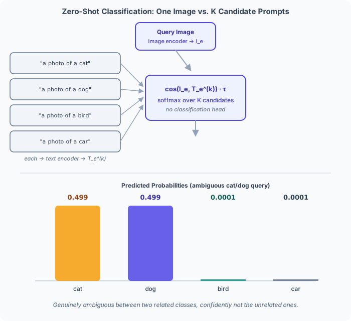
That makes zero-shot classification almost embarrassingly simple: it's Equation (6)'s row computation, run once, with two substitutions. The single "image" is now a genuinely new query image the model never trained on. The "captions" are no longer a training batch's ground-truth pairs — they're a set of hand-written class-name prompts, one per candidate class, with no ground truth at all.
Concretely, in order: pick the classes you want to tell apart and write each one out as a sentence — Figure 7 below uses "a photo of a cat," "a photo of a dog," "a photo of a bird," "a photo of a car." Run every one of those sentences through the already-trained text tower, exactly the way the toy batch's captions were encoded above, producing vectors . Run the query image through the already-trained image tower once, producing a single . Then take cosine similarity between and every , scale by , and softmax across all of them — the identical three-step recipe Equation (6) already used for one row of the training batch's similarity matrix, just with hand-written prompts standing in for that row's training captions:
is however many classes you want to distinguish between right now — it isn't fixed at training time the way ViT's or BERT's fine-tuned classification head fixes their class count into a weight matrix's shape. There's no loss here either, and no target index — Equation (12) is a probability distribution you actually use (typically by taking the argmax), not a training signal. And it's a genuine softmax probability, not an independent per-class likelihood: it's normalized over whichever prompts you happened to write, so adding an eighth candidate class changes every one of the other seven numbers too, even though nothing about the image or those seven prompts changed.
4.2. Worked example: an ambiguous query image
A new image, not one of the four from the training batch — raw projected vector [2, 2, 0, 0], split
evenly between the "cat" and "dog" dimensions instead of favoring one:
query_raw = np.array([2, 2, 0, 0], dtype=float)
query_e = l2norm(query_raw)
print(np.round(query_e, 3))
# [0.707 0.707 0.    0.   ]

# T_e["cat"], T_e["dog"], etc. are the encodings of the full prompts built in the toy
# batch above ("a photo of a cat", "a photo of a dog", ...) — reused here as the K
# zero-shot candidates, unchanged, with no retraining and no access to their labels.
candidates = ["cat", "dog", "bird", "car"]
T_candidates = np.array([T_e[k] for k in candidates])
logits_query = tau * (query_e @ T_candidates.T)
probs_query = softmax(logits_query)

print(np.round(logits_query, 2))
# [8.58 8.58 0.   0.  ]
print(np.round(probs_query, 4))
# [0.4999 0.4999 0.0001 0.0001]
Cosine similarity to "a photo of a cat" and "a photo of a dog" comes out identical — against both, since the query sits exactly halfway between the two directions — so the softmax splits almost exactly 50/50 between them, while "bird" and "car" get essentially none of the probability mass. That's the right answer for a genuinely ambiguous image: not a wrong guess, but honest uncertainty concentrated on the two classes that are actually plausible, with confident rejection of the two that aren't.
4.3. What this replaces
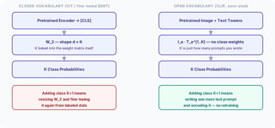
Every classifier built earlier in this series pays a fixed cost to add a class: ViT's classification
head needs resized and retrained; BERT's fine-tuning
step needs a new labeled dataset for the new class alongside the old ones.
CLIP's zero-shot path pays no such cost — a new class is one more string, "a photo of a {new class}", run
through the already-trained text tower once. The paper reports this scheme matching the original supervised
ResNet-50's accuracy on ImageNet without CLIP ever training on a single one of its 1.28 million labeled
examples [1].
Note: the exact wording of the prompt matters more than it might seem. CLIP's own ablations found that bare class names alone (
"cat") underperform full sentence templates ("a photo of a cat"), and that averaging the embeddings from several different templates per class — "prompt engineering," in the paper's own terms — pushes accuracy up further still [1]. This makes sense given what the text tower actually saw during pretraining: real captions scraped from the internet, which read as sentences, not as bare nouns.
That completes the trip from two separately pretrained towers to a single, jointly trained embedding space: a shared projection with L2 normalization turning both towers' outputs into directly comparable unit vectors, a temperature-scaled similarity matrix over a training batch, a symmetric contrastive loss treating every row and column as its own classification problem, and zero-shot classification reusing that exact same row computation at inference time with no head, no fine-tuning, and no fixed class count anywhere in the pipeline.
References
- [1]Radford et al. (2021). Learning Transferable Visual Models From Natural Language Supervision. International Conference on Machine Learning (ICML).
- [2]Dosovitskiy et al. (2020). An Image is Worth 16x16 Words: Transformers for Image Recognition at Scale. International Conference on Learning Representations (ICLR).
- [3]Radford et al. (2019). Language Models are Unsupervised Multitask Learners. OpenAI.
- [4]van den Oord, Li & Vinyals (2018). Representation Learning with Contrastive Predictive Coding.
- [5]Wu et al. (2018). Unsupervised Feature Learning via Non-Parametric Instance Discrimination. IEEE Conference on Computer Vision and Pattern Recognition (CVPR).
- [6]Chen et al. (2020). A Simple Framework for Contrastive Learning of Visual Representations (SimCLR). International Conference on Machine Learning (ICML).