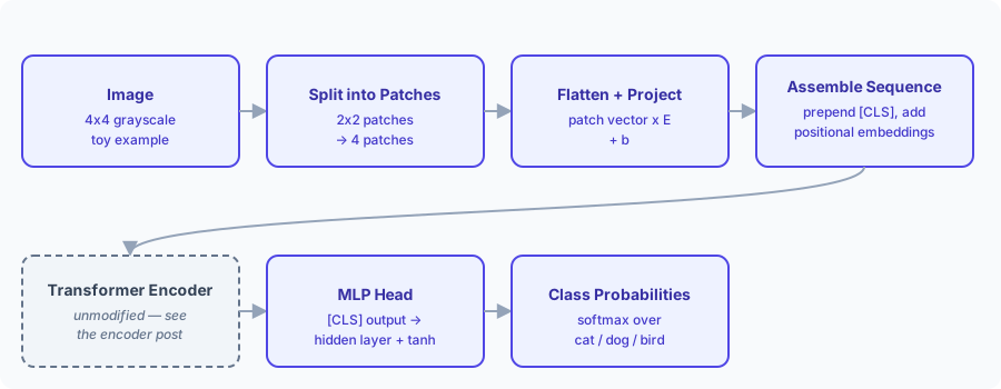
The Transformer was built for language — a sequence of discrete tokens, each one a word or subword. An image has no such sequence: it's a 2D grid of continuous pixel intensities. The Vision Transformer's [1] entire contribution is a recipe for turning that grid into a sequence a Transformer encoder can consume completely unmodified — split the image into small square patches, treat each patch as a "token," and let the exact same encoder architecture do the rest.
Because the encoder itself doesn't change, this post is shorter than the two that came before it. If you haven't read The Transformer Encoder, start there — self-attention, multi-head attention, the feed-forward network, and the residual-plus-normalization wrapper are used here exactly as derived in that post, and none of it is re-derived below. What follows covers only the parts that are genuinely new for images: turning pixels into a sequence, and reading a classification back out.
Contents
This post covers what's specific to the Vision Transformer:
- Patch Embedding — splitting the image into patches, flattening, and linearly projecting each one
- The CLS Token — a learnable token prepended to the sequence for classification
- Positional Embeddings — learnable this time, not the fixed sin/cos formula from the encoder post
- The Transformer Encoder — the same machinery from the earlier post, completely unmodified
- The Classification Head — turning the encoder's output into class probabilities
1. Patch Embedding
Why patches are needed
A Transformer's input has to be a sequence of vectors — that's what self-attention, Q/K/V, all of it, operate on. An image is a grid, not a sequence, so the first job is turning one into the other.
The naive approach — flatten the whole image into one giant vector of individual pixels — falls apart fast. A modest 224x224 color image has over 150,000 pixels; feeding each one in as its own "token" would make self-attention's all-pairs comparison — the encoder post's Self-Attention module — computationally hopeless, and it would throw away the very thing that makes an image an image: nearby pixels belong together.
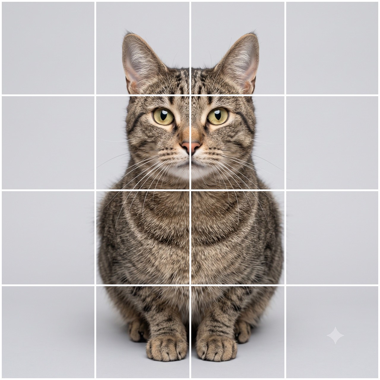
ViT's fix, instead: cut the image into small, fixed-size square patches, and treat each patch — not each pixel — as one token. A 16x16 patch bundles 256 pixels into a single unit; a 224x224 image becomes a much more manageable 14x14 = 196-token sequence.
The toy image
We'll use a tiny 4x4 grayscale image — pixel intensities, not real photo data — small enough to patchify and project entirely by hand:
1  2  5  6
3  4  7  8
9  8  5  4
7  6  3  2
Step 1 — Split into patches
With a patch size of 2x2, the number of patches follows directly from the image size:
With and , Equation (1) gives patches. Splitting the toy image into non-overlapping 2x2 blocks, read left-to-right and top-to-bottom (the same raster order real ViT implementations use):
| Patch | Region | Pixels |
|---|---|---|
| 1 | rows 0-1, cols 0-1 | 1 2 / 3 4 |
| 2 | rows 0-1, cols 2-3 | 5 6 / 7 8 |
| 3 | rows 2-3, cols 0-1 | 9 8 / 7 6 |
| 4 | rows 2-3, cols 2-3 | 5 4 / 3 2 |
import numpy as np

image = np.array([
    [1, 2, 5, 6],
    [3, 4, 7, 8],
    [9, 8, 5, 4],
    [7, 6, 3, 2],
], dtype=float)

patch_size = 2
patches = np.array([
    image[r:r+patch_size, c:c+patch_size].flatten()
    for r in range(0, 4, patch_size)
    for c in range(0, 4, patch_size)
])
print(patches)
# [[1. 2. 3. 4.]
#  [5. 6. 7. 8.]
#  [9. 8. 7. 6.]
#  [5. 4. 3. 2.]]
Step 2 — Flatten each patch
Each 2x2 patch flattens into a 4-element vector, row-major — top row first, then bottom row:
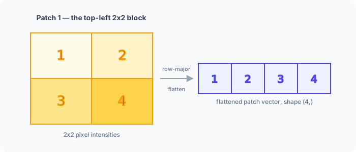
The .flatten() call in the code above already did this — that's exactly why its printed output lines up row-by-row with the patch table.
Step 3 — Linear projection
Flattening alone doesn't produce an embedding — it's still just the original pixel values, rearranged. The actual embedding step is a linear projection: multiply the flattened patch vector by a learned weight matrix and add a learned bias :
Note: most real ViT implementations compute Equation (2) with a single
Conv2dlayer whose kernel size and stride both equal the patch size, rather than an explicit flatten-then-matmul. The two are mathematically identical — a convolution with no overlap and no padding is just "multiply each non-overlapping patch by the same weights" — but theConv2dframing runs faster on GPUs. We use the flatten-then-matmul form here because it's easier to follow by hand.
has shape (flattened patch size) x (embedding dimension) — here, , projecting our 4-pixel patches into the same 4-dimensional embedding space the encoder post used, so the output of this module is a legal input to that post's machinery without any resizing. is a length-4 bias vector, added to every patch the same way.
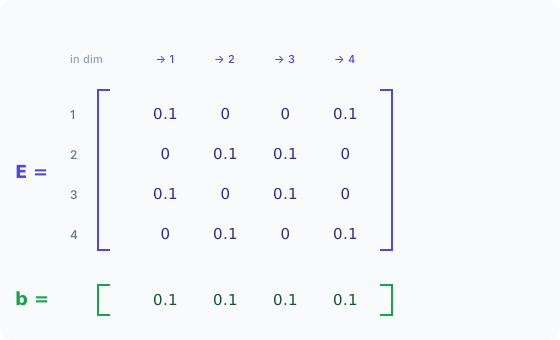
Worked example for patch 1, whose flattened vector is [1, 2, 3, 4]:
(Column-by-column: column 1 is , plus the bias gives — and the same pattern for the other three columns.)
Result — the patch embedding table
The same projection, applied to all four patches:
| Patch | Patch Embedding |
|---|---|
| 1 | [0.5, 0.7, 0.6, 0.6] |
| 2 | [1.3, 1.5, 1.4, 1.4] |
| 3 | [1.7, 1.5, 1.6, 1.6] |
| 4 | [0.9, 0.7, 0.8, 0.8] |
E = np.array([
    [0.1, 0,   0,   0.1],
    [0,   0.1, 0.1, 0  ],
    [0.1, 0,   0.1, 0  ],
    [0,   0.1, 0,   0.1],
])
b_patch = np.array([0.1, 0.1, 0.1, 0.1])

patch_embeddings = patches @ E + b_patch
print(np.round(patch_embeddings, 2))
# [[0.5 0.7 0.6 0.6]
#  [1.3 1.5 1.4 1.4]
#  [1.7 1.5 1.6 1.6]
#  [0.9 0.7 0.8 0.8]]
Four patches in, four 4-dimensional embeddings out — the same shape of result the encoder post's token embedding table produced for its four words. From here on, ViT treats these exactly like token embeddings.
2. The CLS Token
Why classification needs an extra token
Every module in the encoder post produces one output vector per input token — four words in, four output vectors out. That's the right shape for a task like next-word prediction, where every position needs its own answer. Classification is different: "what's in this image" needs exactly one answer for the whole sequence, not four.
ViT borrows a trick from BERT [3]: prepend one extra, purely learnable embedding — called [CLS], short for "classification" — to the front of the sequence, before it ever reaches the encoder. It doesn't correspond to any patch; it starts from a generic, trainable vector with no fixed meaning. As the sequence passes through self-attention, [CLS] attends to (and gathers information from) every patch — and every patch can attend back to it — so by the time the sequence reaches the last encoder block, [CLS]'s output vector has absorbed a summary of the whole image. That single vector is what the classification head — covered later in this post — reads.
Note:
[CLS]isn't the only option. The original ViT paper also tried skipping it entirely and instead average-pooling all the patch outputs together, and found the two approaches perform comparably with the right learning-rate tuning [1].[CLS]is used here — and in most ViT code you'll encounter — mainly for continuity with BERT.
Step — Prepend to the sequence
Give [CLS] a small hand-picked starting vector, [0.2, 0.2, 0.2, 0.2], and place it at position 0, ahead of the four patch embeddings from the Patch Embedding step above:
| Position | Token | Embedding |
|---|---|---|
| 0 | [CLS] | [0.2, 0.2, 0.2, 0.2] |
| 1 | patch 1 | [0.5, 0.7, 0.6, 0.6] |
| 2 | patch 2 | [1.3, 1.5, 1.4, 1.4] |
| 3 | patch 3 | [1.7, 1.5, 1.6, 1.6] |
| 4 | patch 4 | [0.9, 0.7, 0.8, 0.8] |
cls_token = np.array([0.2, 0.2, 0.2, 0.2])
seq = np.vstack([cls_token, patch_embeddings])
print(seq)
# [[0.2 0.2 0.2 0.2]
#  [0.5 0.7 0.6 0.6]
#  [1.3 1.5 1.4 1.4]
#  [1.7 1.5 1.6 1.6]
#  [0.9 0.7 0.8 0.8]]
Five rows now, not four — one [CLS] plus four patches. Every module downstream, starting with positional embeddings, operates on this 5-token sequence.
3. Positional Embeddings
Why position still matters
Self-attention has no built-in sense of order — the encoder post's Positional Encoding module made exactly this point for a sentence, and the same problem shows up here for an image. Swap two patches' positions in the sequence and self-attention, on its own, can't tell the difference; it just sees two vectors trading places. Some signal has to be added that says "this embedding belongs at this specific position."
Learnable vs. fixed positional embeddings
The encoder post's answer was a fixed formula from the original Transformer paper [2] — Equation (1) and Equation (2), sine and cosine waves at a range of frequencies, no learning involved. ViT does the same job differently: instead of a formula, it uses a learnable positional embedding table — one trainable vector per position, initialized randomly like any other weight and updated by backpropagation during training. There's no sin, no cos, no term anywhere — just vectors (one per patch, plus one for [CLS]) that the model learns are useful.
Note: this fixed-size table is why ViT needs a fixed input resolution. The patch projection from Equation (2) doesn't care how many patches there are — it's applied one patch at a time, so the same matrix works whether an image splits into 4 patches or 4,000. is different: it has exactly rows, one per position, so has to stay fixed for the table to line up. In practice, this is why input images are resized or center-cropped to a single canonical resolution (224x224 is the common choice) before patchifying — changing the resolution changes via Equation (1), and a positional embedding table sized for the old no longer applies.
Note: the original ViT paper ran the comparison directly [1] — 1D learnable positional embeddings (what's used below), a 2D-aware learnable variant that treats row and column position separately, and relative positional embeddings. All three landed within a fraction of a percent of each other on final accuracy. 1D learnable wins by default not because it's best, but because it's simplest — one lookup table, nothing image-specific baked in.
Step — Add to the sequence
A hand-picked 5x4 positional embedding table, one row per position, added elementwise to the sequence built in the CLS Token step above:
| Position | Positional Embedding |
|---|---|
| 0 | [0.05, 0.05, 0.05, 0.05] |
| 1 | [0.10, 0.00, 0.00, 0.10] |
| 2 | [0.00, 0.10, 0.10, 0.00] |
| 3 | [0.10, 0.10, 0.00, 0.00] |
| 4 | [0.00, 0.00, 0.10, 0.10] |
![Diagram prepending the [CLS] token and adding positional embeddings](/images/understanding-vit/cls-and-positional-embedding.svg)
Result — the final input sequence
| Position | Token | + Positional | = Final Embedding |
|---|---|---|---|
| 0 | [CLS] | [0.05, 0.05, 0.05, 0.05] | [0.25, 0.25, 0.25, 0.25] |
| 1 | patch 1 | [0.10, 0.00, 0.00, 0.10] | [0.60, 0.70, 0.60, 0.70] |
| 2 | patch 2 | [0.00, 0.10, 0.10, 0.00] | [1.30, 1.60, 1.50, 1.40] |
| 3 | patch 3 | [0.10, 0.10, 0.00, 0.00] | [1.80, 1.60, 1.60, 1.60] |
| 4 | patch 4 | [0.00, 0.00, 0.10, 0.10] | [0.90, 0.70, 0.90, 0.90] |
pos_emb = np.array([
    [0.05, 0.05, 0.05, 0.05],
    [0.10, 0.00, 0.00, 0.10],
    [0.00, 0.10, 0.10, 0.00],
    [0.10, 0.10, 0.00, 0.00],
    [0.00, 0.00, 0.10, 0.10],
])

final_seq = seq + pos_emb
print(np.round(final_seq, 2))
# [[0.25 0.25 0.25 0.25]
#  [0.6  0.7  0.6  0.7 ]
#  [1.3  1.6  1.5  1.4 ]
#  [1.8  1.6  1.6  1.6 ]
#  [0.9  0.7  0.9  0.9 ]]
This 5x4 matrix, final_seq, is exactly what feeds into the Transformer encoder next — five tokens, four dimensions each, the identical shape the encoder post's Query/Key/Value, Self-Attention, Multi-Head Attention, and Feed-Forward Network modules were built to consume.
4. The Transformer Encoder
Feeding the sequence in
final_seq from the Positional Embeddings step above is a legal input to The Transformer Encoder exactly as written — Q/K/V projection, self-attention (Equation (7)), multi-head attention, the feed-forward network, and the residual-plus-normalization wrapper around each sub-layer, none of it changed. Every one of final_seq's five rows plays the same role a token's position-aware embedding played in that post; the encoder has no idea, and no need to know, that four of these five "tokens" actually came from image patches.
What changes, what doesn't
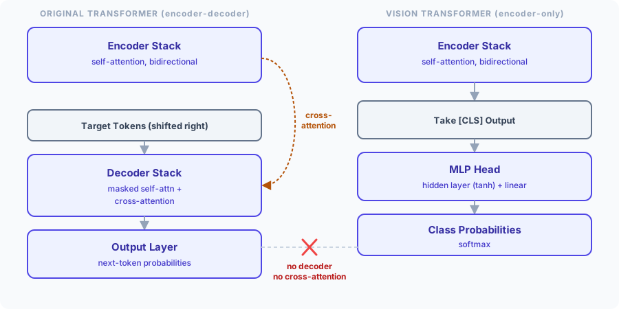
Nothing in the mechanism itself is vision-specific. Two things are genuinely different from the encoder post's language example, and both are about how the mechanism is used, not the mechanism itself:
- No causal mask. The encoder post's Self-Attention module introduced causal masking — Equation (8) and Equation (9) — as something a decoder-style model needs, so it can't peek at future tokens. ViT never applies it: every patch, and
[CLS], can attend to every other patch and to[CLS]right from the first block. There's no "future" in an image the way there's a future word in a sentence — all patches exist simultaneously, so ViT's self-attention is fully bidirectional, the same as an encoder like BERT. - Only one output row matters downstream. The encoder produces five context-aware output vectors, one per input row — but the classification head, covered next, only reads the row at position 0,
[CLS]'s. The other four rows did real work along the way (every attention computation mixes information across all five), but nothing downstream consumes them directly.
Both of those are usage differences within the same encoder module — nothing about the model's overall shape has changed yet. The bigger structural difference is what's entirely absent: ViT has no decoder and no cross-attention. The diagram below lines the two architectures up side by side to make that explicit.
5. The Classification Head
From encoder output to class scores
Running final_seq through the encoder stack isn't repeated here — it's exactly the computation already worked through, module by module, in the linked post. So this module starts from a clearly-labeled hypothetical: suppose that, after passing through the encoder blocks, the [CLS] token's final output is
(a stand-in for whatever number actually falls out of running the full encoder — the point of this module is what happens after that, which is genuinely new.)
The formula
A small two-layer MLP turns [CLS]'s output into class probabilities — a hidden layer with a nonlinearity, then a linear layer down to one score per class, then softmax:
Note: the original ViT paper's classification head actually differs between training phases: pretraining uses a hidden layer with , exactly Equation (5), while fine-tuning on the target task drops down to a single linear layer with no hidden layer at all. We use the two-layer version here since it makes for a slightly more complete worked example — the same shape of computation as the encoder post's Feed-Forward Network module, just ending in softmax instead of being fed back into another block.
Step 1 — Hidden layer
is here (embedding dimension in, hidden dimension out — kept equal just to keep the arithmetic small); :
Step 2 — Logits and softmax
is — three toy classes, cat, dog, bird (a light callback to the encoder post's toy vocabulary, which also had "dog" and "cat" in it); :
| cat | dog | bird | |
|---|---|---|---|
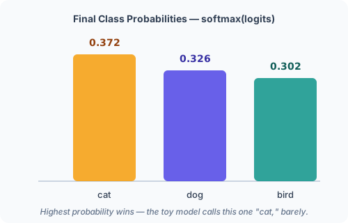
| logits | 0.317 | 0.186 | 0.108 |
| softmax probability | 0.372 | 0.326 | 0.302 |
z_cls = np.array([0.4, 1.1, 0.7, 0.3])

W1 = np.array([
    [0.3, 0,   0.2, 0  ],
    [0,   0.3, 0,   0.2],
    [0.2, 0,   0.3, 0  ],
    [0,   0.2, 0,   0.3],
])
b1 = np.array([0.0, 0.0, 0.0, 0.0])

W2 = np.array([
    [1.0,  0.2, -0.5],
    [0.3, -0.4,  0.8],
    [-0.6, 0.9,  0.1],
    [0.4,  0.1, -0.3],
])
b2 = np.array([0.0, 0.0, 0.0])

hidden = np.tanh(z_cls @ W1 + b1)
logits = hidden @ W2 + b2

exp_logits = np.exp(logits - logits.max())
probs = exp_logits / exp_logits.sum()

print(np.round(logits, 3))
# [0.317 0.186 0.108]
print(np.round(probs, 3))
# [0.372 0.326 0.302]   # cat, dog, bird
Result — class probabilities
cat edges out dog and bird, 0.372 to 0.326 to 0.302 — a close call, which makes sense: with hand-picked weights and a made-up z_cls, there's no reason to expect a confident prediction. In a trained model, this same pipeline — patchify, embed, prepend [CLS], add positional embeddings, run through the encoder, read out [CLS], apply the classification head — is what turns a photograph into "97% cat."
That's the complete Vision Transformer pipeline: an image in, patches out, a sequence through an entirely unmodified Transformer encoder, and a classification back out the other end. What's left out of scope here — fine-tuning at a higher resolution than pretraining used, hybrid CNN-ViT architectures, and data-efficient training via distillation [4] — is where the current ViT literature spends most of its effort, but all of it builds on exactly the pipeline worked through above.
References
- [1]Dosovitskiy et al. (2020). An Image is Worth 16x16 Words: Transformers for Image Recognition at Scale. International Conference on Learning Representations (ICLR).
- [2]Vaswani et al. (2017). Attention Is All You Need. Conference on Neural Information Processing Systems (NeurIPS).
- [3]Devlin et al. (2018). BERT: Pre-training of Deep Bidirectional Transformers for Language Understanding. Conference of the North American Chapter of the Association for Computational Linguistics: Human Language Technologies (NAACL-HLT).
- [4]Touvron et al. (2020). Training data-efficient image transformers & distillation through attention. International Conference on Machine Learning (ICML).