NeRF made a scene into a function: no stored geometry anywhere, just the weights of a small MLP, queryable at any continuous point. That continuity bought a lot — but it came with a bill due at render time, paid in full for every single pixel: up to roughly 192 network forward passes per pixel, on the order of per frame, because the only way to find out what's at a point is to ask the network. 3D Gaussian Splatting [1] keeps NeRF's core rendering idea — composite weighted contributions along a line of sight — and throws out the part that was actually expensive: the network. What's left, once the MLP is gone, is a scene stored as an explicit, finite collection of primitives again, the way classical reconstruction always did it. The primitives are just smoother now.
This post works through what those primitives are and how a photograph gets rendered from them: what a 3D Gaussian stores, how its covariance is built so it's always a valid shape, how it gets projected onto the image plane through a real camera, the alpha-compositing equation that turns a stack of overlapping Gaussians into a pixel — the same equation NeRF used, structurally unchanged — and the tile-based sorting trick and the densify/split/prune training loop that make the whole thing run in real time.
Contents
- From a Queried Field Back to Stored Primitives — what going explicit again actually buys, and what it costs
- A 3D Gaussian as a Primitive — the handful of numbers each Gaussian stores, and the falloff function they define
- Parameterizing a Valid Covariance — why Σ is never optimized directly, and the scale-and-rotation decomposition that replaces it
- Splatting: Projecting a 3D Gaussian to Screen Space — the camera Jacobian that turns a 3D ellipsoid into a 2D ellipse, worked by hand on a real Gaussian
- Point-Based Alpha Blending — NeRF's compositing equation again, now summing over sorted primitives instead of ray samples
- Tile-Based Differentiable Rasterization — how splatting stays fast: one depth sort shared by every pixel in a tile
- Spherical Harmonics for View-Dependent Color — the non-neural analogue of NeRF's positional encoding of viewing direction
- Initialization and Adaptive Density Control — growing a scene from a sparse point cloud by cloning, splitting, and pruning Gaussians during training
- Training Loss, Cost, and What Gaussian Splatting Buys — the photometric loss, and the actual trade being made against NeRF's per-pixel network cost
- Putting It Together: A Minimal Reference Implementation — every piece above, assembled into a small, plain, brute-force forward renderer
1. From a Queried Field Back to Stored Primitives
1.1 What the implicit field was paying for
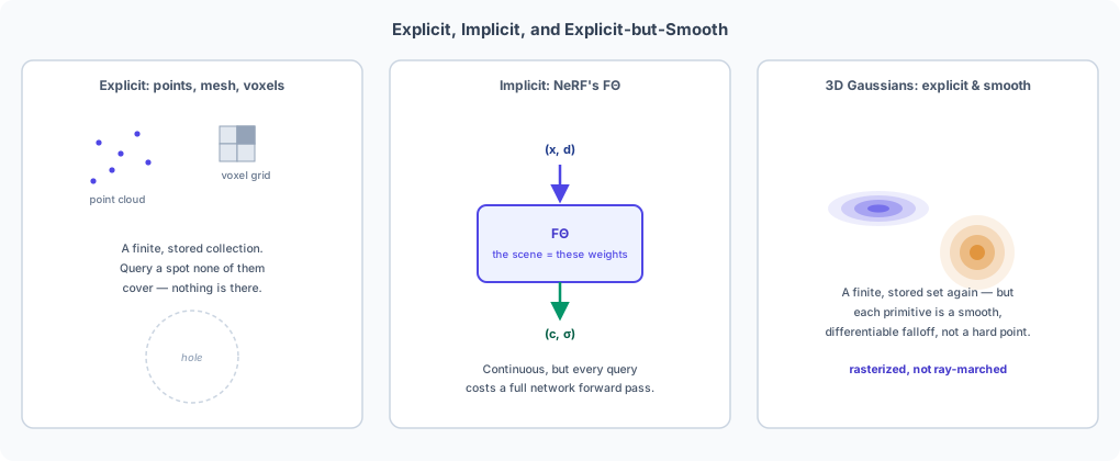
NeRF's whole appeal was continuity: nothing about the scene is discretized until the very last step, so the field can be queried at any , including points nothing in training ever landed on exactly. The cost section of that post worked out exactly what that buys — every pixel of every frame requires marching a ray through the field and evaluating a neural network at every sample along it, because there's no stored geometry to look up, only a function to ask, over and over.
1.2 Going back to explicit, without going back to rigid
3D Gaussian Splatting walks that trade back the other direction, but not all the way back to where classical reconstruction started. A scene becomes a finite set — typically hundreds of thousands to a few million — of 3D Gaussians, each one an explicit, stored primitive with its own position and shape, much closer in spirit to a point cloud than to a neural field. What doesn't come back is the rigidity: a point in a point cloud is either there or it isn't, but a 3D Gaussian is a smooth, everywhere-differentiable function of space, with soft, overlapping falloff instead of a hard boundary. That's what keeps the whole pipeline trainable by gradient descent, the same property Section 8.2 of the NeRF post pinned on the smoothness of — nothing here is a hard if-else either.
2. A 3D Gaussian as a Primitive
2.1 What each primitive stores
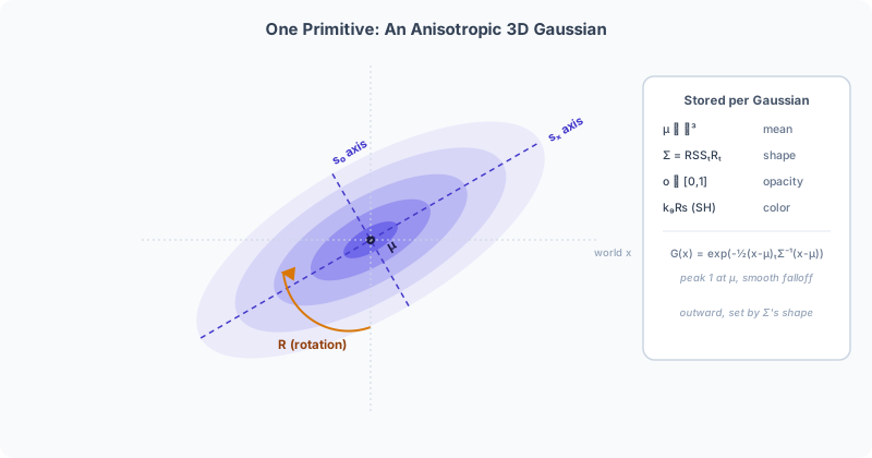
Every Gaussian carries a small, fixed set of numbers, and unlike NeRF's — weights a network forward pass reads through — these numbers are the free parameters: training (Section 9) runs gradient descent directly on them, comparing a rendered image against a real photograph and updating each Gaussian's own numbers to reduce that error, with no network standing in between. Per Gaussian: a mean (its center), a covariance (its size and orientation — Section 3 covers how this is actually parameterized, since handing gradient descent a raw to update directly turns out to be a problem), an opacity , and a color that can depend on viewing direction, stored as a small set of spherical-harmonic coefficients rather than raw RGB (Section 7). Position, shape, opacity, and color, all stored directly per-primitive — nothing here is read out of a network.
2.2 The shape function
The covariance defines a falloff around the mean, the multivariate Gaussian density shape, evaluated at any 3D point :
Unlike NeRF's , Equation (1), isn't an absorption rate with its own physical units — it's a unitless shape, normalized so at the center and falling off smoothly with Mahalanobis distance, the same distance metric a multivariate Gaussian PDF always uses, just without the PDF's own normalizing constant in front (there's no need for to integrate to 1 — it isn't a probability density here, only a weighting function).
Note: Mahalanobis distance is just squared Euclidean distance, , generalized to account for a shape instead of assuming a perfect sphere: swapping in , , rescales each direction by how far the ellipsoid actually extends that way. A point sitting right on the tip of a long axis and a point sitting on the flat side of a short axis can be the same Mahalanobis distance from even though the long-axis point is farther away in raw Euclidean terms — which is exactly what should happen: Equation (1) ought to fall off at the same rate in every direction the ellipsoid was actually built to stretch in, not treat a point just outside a thin axis as "closer" than one still comfortably inside a long one.
and are separate numbers for a reason that matters later: sets how opaque the primitive is at its core — fully transparent, fully opaque — and , peaking at at the mean and falling toward away from it, shapes how much of that core opacity actually reaches a given point. Section 5 multiplies them back together to get an actual per-pixel alpha.
3. Parameterizing a Valid Covariance
3.1 Why Σ is never handed to gradient descent directly
Section 2.1 established that is a free parameter gradient descent updates on every training step, the same as and — but can't be treated as just nine independent numbers the way those two can, because it has to stay symmetric and positive semi-definite for Equation (1) to mean anything — a covariance with a negative eigenvalue isn't a valid shape at all. Handing a raw matrix to gradient descent and hoping every update keeps both properties intact is fragile: nothing about an ordinary gradient step respects either constraint, and it takes only one bad step to produce a that can't be inverted.
3.2 Scale and rotation instead
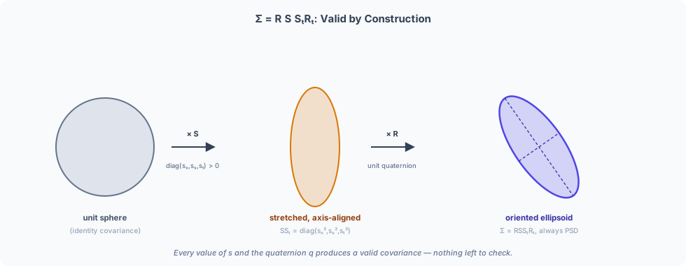
The fix decomposes into a piece that's positive by construction and a piece that's orthogonal by construction, and multiplies them together:
is a diagonal scale matrix — three positive numbers, but never handed to gradient descent as itself. What's actually stored and updated is , an unconstrained log-scale, with computed fresh on every forward pass:
A gradient step is free to push to, say, — still an ordinary, unconstrained real number — and comes out positive regardless, just very small; there is no raw value of that exponentiates to zero or a negative number.
gets the same treatment. The parameter gradient descent actually optimizes is a raw 4-vector
— four unconstrained numbers, no different in kind from —
and the unit quaternion that quat_to_rotmat turns into is computed fresh on every forward
pass by normalizing it:
holds automatically after that division, for any nonzero whatsoever, so comes out orthogonal — a valid rotation — regardless of what gradient descent has done to 's four raw components. is positive definite for any nonzero scale, and conjugating a positive definite matrix by any rotation preserves positive definiteness — so Equation (2) produces a valid for every value of and , with no constraint left to violate. Seven numbers — three for , four for — replace what would otherwise be six independent entries of a symmetric , and never once need to be checked for validity.
A worked example: a Gaussian scaled thin along one local axis and long along another, , rotated about the world -axis:
import numpy as np

def quat_to_rotmat(q):
    w, x, y, z = q
    return np.array([
        [1 - 2*(y*y + z*z), 2*(x*y - w*z),     2*(x*z + w*y)],
        [2*(x*y + w*z),     1 - 2*(x*x + z*z), 2*(y*z - w*x)],
        [2*(x*z - w*y),     2*(y*z + w*x),     1 - 2*(x*x + y*y)],
    ])

s = np.array([0.03, 0.15, 0.20])
angle = np.deg2rad(45)
q = np.array([np.cos(angle / 2), 0.0, 0.0, np.sin(angle / 2)])  # rotate about z

R = quat_to_rotmat(q)
S = np.diag(s)
Sigma = R @ S @ S.T @ R.T

print(np.round(Sigma, 4))
# [[ 0.0117 -0.0108  0.    ]
#  [-0.0108  0.0117  0.    ]
#  [ 0.      0.      0.04  ]]
print(np.round(sorted(np.linalg.eigvalsh(Sigma)), 4))
# [0.0009 0.0225 0.04  ]  -- exactly s**2, sorted: the rotation never changed the shape,
#                            only the orientation the off-diagonal terms now encode.
The nonzero off-diagonal entries, in both the and slots, are exactly what a rotation does to a diagonal covariance: they encode "this ellipsoid's axes don't line up with the world axes anymore," while the eigenvalues — the true, rotation-independent extent along each principal axis — stay identically . This same is reused directly in Section 4's projection example.
4. Splatting: Projecting a 3D Gaussian to Screen Space
4.1 Two transforms, one exact and one approximated
Getting a Gaussian onto the screen runs its mean and its covariance through the camera in two stages: a rigid transform from world space into camera space, then a perspective projection from camera space onto the image plane. The mean passes through both stages exactly — nothing is approximated for a single point. Camera space is defined by a rotation and a translation together, the camera's viewing transform:
is the camera's rotation, its translation. then finishes the mean's trip to the screen with a second step that's still exact — dividing by depth through the camera's pinhole projection:
No approximation is needed here either: is an ordinary, well-defined function, and evaluating it exactly at one single point costs nothing — a single point never needed linearizing in the first place. and the covariance formula coming up next are two separate computations that only happen to share the same : depends on directly, through , while (below) will turn out not to need as a term of its own at all.
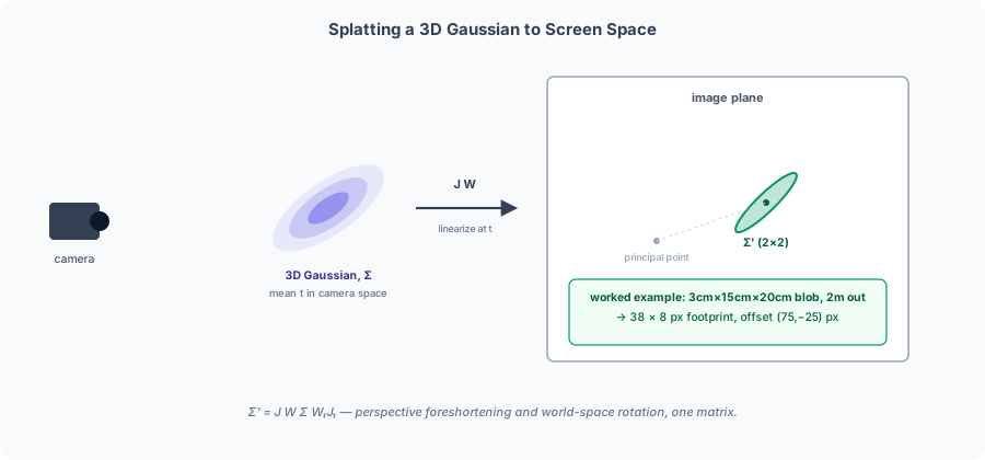
is where an exact answer runs out. It isn't a single point, it's an entire spread of points around , and there's no way to push that whole spread through 's division by depth and still get an exact Gaussian back out — which is exactly what is for:
never needs inside this formula, for the same reason above didn't need it added in: is built entirely out of differences around the mean, and a constant translation cancels out of any difference — , nowhere in it — which is also the entire reason appears here as a plain rotation rather than the matrix a view transform usually is. Translation still reaches indirectly, though, since (Section 4.2 derives it) is itself a function of : move the camera and changes, so changes too (closer means more foreshortening), even though is never a term added anywhere inside directly.
4.2 Deriving J: linearizing the projection at the mean
Reusing from Section 4.1: pushing an entire covariance through it exactly has no answer, so the standard fix for propagating a distribution through any smooth nonlinear map applies instead — the technique this whole splatting step is named after, tracing back to EWA (elliptical weighted average) splatting [2] — replace the map with its first-order Taylor expansion around the mean, the curved surface swapped for its tangent plane, accurate precisely because the region the Gaussian has any real weight in is small:
is nothing more than a matrix of partial derivatives: differentiate and with respect to each of , , (the quotient rule supplies the and terms), pad with a zero row since depth itself is dropped after projection, and the result is exactly the matrix Equation (7) needs:
The bottom row is zero for the same reason it was padded in: depth is discarded after projection, so 's top-left block is the only part that ends up describing an on-screen footprint. scaling the first two rows is exactly perspective foreshortening (farther Gaussians shrink), and the , terms are the shear that a Gaussian off to the side of the image picks up purely from projection geometry — nothing to do with the Gaussian's own orientation. is a fixed matrix once evaluated at , not a function of anymore, so it's linear exactly where it's used — and a linear map pushed through a Gaussian stays a Gaussian, which is what lets Equation (7) transform by simple conjugation instead of needing an integral.
4.3 Projecting Section 3's Gaussian through a real camera
Take Section 3's exact , place it at world position in front of an identity-view camera (, so camera space equals world space here) with focal length pixels:
Sigma = np.array([
    [ 0.0117, -0.0108, 0.0],
    [-0.0108,  0.0117, 0.0],
    [ 0.0,     0.0,    0.04],
])
W = np.eye(3)
fx, fy = 500.0, 500.0
t0, t1, t2 = 0.3, -0.1, 2.0

J = np.array([
    [fx / t2, 0.0,     -fx * t0 / t2**2],
    [0.0,     fy / t2, -fy * t1 / t2**2],
    [0.0,     0.0,      0.0],
])

Sigma_2d = (J @ W @ Sigma @ W.T @ J.T)[:2, :2]
eigvals, eigvecs = np.linalg.eigh(Sigma_2d)
order = np.argsort(eigvals)[::-1]
radii_px = np.sqrt(eigvals[order])
angle_deg = np.degrees(np.arctan2(*eigvecs[::-1, order[0]]))

print(np.round(Sigma_2d, 2))
# [[ 787.5 -693.75]
#  [-693.75  737.5 ]]
print("1-sigma radii (px):", np.round(radii_px, 1))       # [38.2  8.3]
print("major-axis angle (deg):", round(angle_deg, 1))     # 136.0
print("projected pixel offset:", fx * t0 / t2, fy * t1 / t2)  # (75.0, -25.0)
Two genuinely separate results come out of this. The position, pixels off the principal point, is just Equation (6) — , the mean's own exact projection — and it would move if (folded into here since and the camera sits at the origin) did, even though nothing about computing it touched or at all. The shape, the pixel ellipse tilted from the pixel -axis (equivalently — an ellipse's axis has no arrowhead, so the two describe the same tilt), is the entirely separate job of Equation (7) — the perspective shear from and the world-space rotation from Section 3 both baked into one matrix, with no separate step for "figure out which way the ellipse should tilt on screen," and no dependence on beyond what already reached it through . Nothing about this step has touched a pixel, an opacity, or a color yet, and it doesn't depend on any other Gaussian in the scene either — splatting produces exactly two numbers per Gaussian, a screen-space mean and a , ready to be evaluated wherever rendering actually needs them. That's where Section 5 picks up.
5. Point-Based Alpha Blending
5.1 The same compositing equation, different source
NeRF's volume rendering integral reduces, once discretized, to Equation (5) — sort samples along a ray, composite front-to-back with weights . Gaussian Splatting reaches the same form of equation from a different starting point: instead of samples along one ray per pixel, it's primitives sorted by depth, evaluated directly at the pixel. Each Gaussian contributes its own projected mean (Equation (6)) and covariance (Equation (7)), which together give a per-Gaussian 2D shape function, — Equation (1) restricted to the screen plane, with in place of and in place of . Evaluating at a specific pixel , and multiplying by opacity, gives that Gaussian's local alpha at that pixel:
sets the ceiling — how opaque this Gaussian is at its very center — and scales that down according to how far sits from , in the metric defines. Sorted front-to-back by each Gaussian's own depth (Section 6.1 makes precise what "depth" means here), exactly NeRF's alpha-compositing weight structure returns:
Writing makes the match to Equation (5) exact: , the identical "over" compositing operator, walked over a sorted list of primitives instead of a sorted list of ray samples. What changed between the two posts is entirely upstream of this equation — where and come from — not the compositing rule itself.
5.2 A four-splat toy pixel, by hand
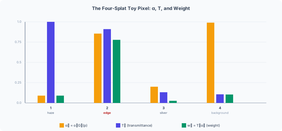
Four Gaussians happen to overlap one pixel, sorted nearest-to-farthest: a faint haze in front, a near-opaque object edge, a thin sliver crossing behind it, and a fully opaque background. runs from fully transparent at to fully opaque at , so the haze's reads as a thin, barely-there wisp rather than a dense one — a dense fog would sit up near , closer to the background's . peaks at exactly at this splat's own projected center and falls toward out in its tails, so every here landing between and means the pixel sits fairly close to each splat's own center relative to its footprint — none of these four is grazing the pixel from way out in its tail:
| reading | |||
|---|---|---|---|
| 1 | 0.10 | 0.90 | faint haze, close to camera |
| 2 | 0.90 | 0.95 | a near-opaque object edge |
| 3 | 0.40 | 0.50 | a thin sliver, partially behind it |
| 4 | 1.00 | 0.99 | fully opaque background |
o = np.array([0.10, 0.90, 0.40, 1.00])
G = np.array([0.90, 0.95, 0.50, 0.99])
c = np.array([0.30, 0.80, 0.50, 0.10])

alpha = o * G
T = np.concatenate([[1.0], np.cumprod(1.0 - alpha)[:-1]])
weights = T * alpha
C_hat = np.sum(weights * c)

print("alpha  ", np.round(alpha, 3))    # [0.09  0.855 0.2   0.99 ]
print("T      ", np.round(T, 3))        # [1.    0.91  0.132 0.106]
print("weights", np.round(weights, 3))  # [0.09  0.778 0.026 0.104]
print("C_hat  ", round(float(C_hat), 3))  # 0.673
Splat 2 dominates the pixel, contributing weight out of a total that sums to essentially . Splat 4, the fully opaque background, has — the highest opacity of any splat here — and still only contributes , because by the time the ray of compositing reaches it, : 89% of the pixel's "light" has already been spent on splats 1 and 2. Nothing about overrides that; opacity only ever controls how much of the remaining transmittance a splat consumes, exactly the reading Section 4.2 of the NeRF post gave sample 4 of its own toy ray — occlusion falling straight out of the compositing equation, not a separate visibility test bolted on.
6. Tile-Based Differentiable Rasterization
6.1 One sort, shared by every pixel in a tile
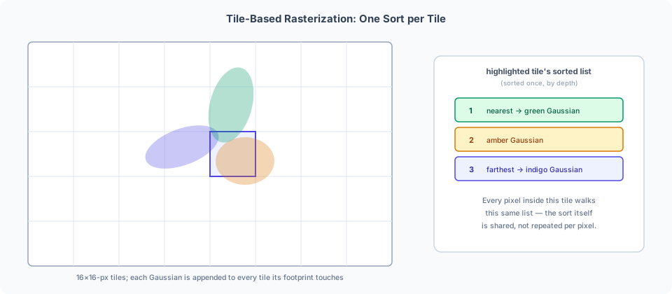
A Gaussian has no surface, so "its depth" isn't literally defined the way it is for a mesh triangle — what gets sorted is a single scalar per Gaussian, the camera-space depth of its own mean (the same already computed for Equation (5) and Equation (6)), treating the whole blob as if it sat at that one depth and ignoring how far it actually extends in front of and behind it. Equation (11) needs the Gaussians overlapping a given pixel sorted by that depth — but resorting from scratch at every one of an image's million-plus pixels, each potentially touching dozens of overlapping splats, is its own expensive bottleneck. The screen is instead divided into a coarse grid of -pixel tiles. Each Gaussian's screen-space footprint (its bounding box, cheaply available from Section 4.3's projected radii) is checked against every tile it overlaps, and a reference to that Gaussian is appended to each tile's list — one Gaussian can and often does land in several tiles' lists at once. Every tile's list gets depth-sorted exactly once, and then every pixel inside that tile walks the same sorted list, evaluating Equation (10) and accumulating Equation (11) independently — the sort itself is amortized across every pixel in the tile instead of repeated per pixel.
def assign_to_tiles(mean_px, radius_px, tile_size=16, image_size=(1920, 1080)):
    x0 = max(0, int((mean_px[0] - radius_px) // tile_size))
    x1 = min(image_size[0] // tile_size, int((mean_px[0] + radius_px) // tile_size) + 1)
    y0 = max(0, int((mean_px[1] - radius_px) // tile_size))
    y1 = min(image_size[1] // tile_size, int((mean_px[1] + radius_px) // tile_size) + 1)
    return [(tx, ty) for ty in range(y0, y1) for tx in range(x0, x1)]

# Section 4.3's Gaussian: mean offset (75, -25) from principal point, ~38 px major radius
tiles = assign_to_tiles((960 + 75, 540 - 25), radius_px=38)
print(len(tiles), "tiles touched:", tiles[:4], "...")
6.2 Staying differentiable
Nothing about tiling or sorting breaks differentiability: the forward pass composites exactly Equation (11), tile by tile, and the backward pass walks the same sorted lists in reverse, accumulating gradients into each contributing Gaussian's , (through and ), , and color coefficients — the same principle NeRF's Section 8.2 leaned on to backpropagate a rendering error all the way into , just with per-primitive parameters standing in for network weights. This is the piece that actually needs a custom CUDA kernel to be fast in practice — the tiling, sorting, and per-tile compositing described here, forward and backward, is exactly the workload the original implementation hand-writes rather than expressing in a generic autodiff framework.
An updated or changes and, downstream of it, the projected radius Section 6.1 bins into tiles with — but the backward pass never patches the tile lists it just walked. Tile assignment and the per-tile sort are recomputed completely from scratch on the next forward pass, from whatever and the optimizer step just produced, exactly the way Section 6.1 already described it — the same full rebuild happens on every rendered frame regardless of whether any Gaussian's own parameters changed at all, since a new camera view alone already changes every projected footprint and depth order.
7. Spherical Harmonics for View-Dependent Color
7.1 A non-neural analogue of positional encoding
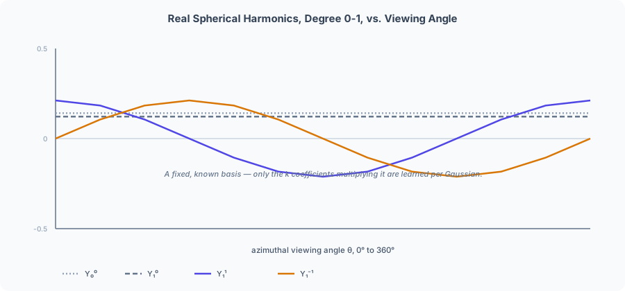
NeRF let color depend on viewing direction by concatenating an encoded direction, Equation (6), into an MLP and letting the network figure out the mapping. There's no MLP here to hand that job to, so each Gaussian instead stores a small, fixed set of spherical-harmonic coefficients per color channel — R, G, and B each get their own independent set — and viewing direction is projected onto that basis directly at query time:
are the real spherical harmonic basis functions — fixed, known in closed form, not learned — and are the only learned quantities, one small coefficient vector per Gaussian per channel. The paper uses degree (4 bands, ), giving coefficients per channel, 48 total for RGB — replacing NeRF's 128-unit hidden layer and final projection (Section 7.1 of that post) with a fixed-basis dot product. Not every coefficient is active from the start of training, either: every Gaussian begins with only the constant term, and one further band is unlocked every 1000 iterations until all four are in play — color starts view-independent and only gradually earns the ability to vary with direction, rather than being handed the full basis on iteration one.
7.2 Two viewing directions, one set of coefficients
The lowest two bands, and — 4 of the paper's 16 basis functions per channel — have simple closed forms: , , , . and add 5 and 7 more basis functions respectively, each still closed-form but algebraically more involved (products of direction components rather than a single linear term), omitted here for space. The worked example below truncates to just these first 4 — a degree-1 toy, not the paper's full degree-3 — so is a 4-element vector rather than the real 16-element one; and would be two more, independently learned vectors of the same length, unrelated to by anything but sharing the same Gaussian. Fix one Gaussian's red-channel coefficients and evaluate from two different viewing directions:
def sh_degree1(d):
    x, y, z = d
    return np.array([0.282095, 0.488603 * y, 0.488603 * z, 0.488603 * x])

k_R = np.array([0.9, 0.05, -0.10, 0.20])  # fixed, learned once per Gaussian

d1 = np.array([0.3, 0.4, 0.866]); d1 /= np.linalg.norm(d1)
d2 = np.array([-0.6, -0.2, 0.7]); d2 /= np.linalg.norm(d2)

c_R1 = max(0.0, np.dot(k_R, sh_degree1(d1)) + 0.5)
c_R2 = max(0.0, np.dot(k_R, sh_degree1(d2)) + 0.5)
print(round(c_R1, 3), round(c_R2, 3))  # 0.751 0.65
Same Gaussian, same stored , and the red channel still shifts from to purely because changed — a specular-like, view-dependent color out of a closed-form basis evaluation, no forward pass required.
8. Initialization and Adaptive Density Control
8.1 Starting from a point cloud, not from nothing
Training starts from the sparse 3D point cloud a structure-from-motion pipeline like COLMAP [4] already produces from the same posed photographs — the identical starting material NeRF's training section mentioned only in passing, since NeRF needs camera poses from that pipeline but throws the points themselves away. Gaussian Splatting keeps them: every SfM point becomes one small, initially isotropic Gaussian. That's the return, foreshadowed at the end of the NeRF post, to "representations classical reconstruction already produces" — just as a starting point this time, not a final answer.
8.2 Cloning, splitting, and pruning during training
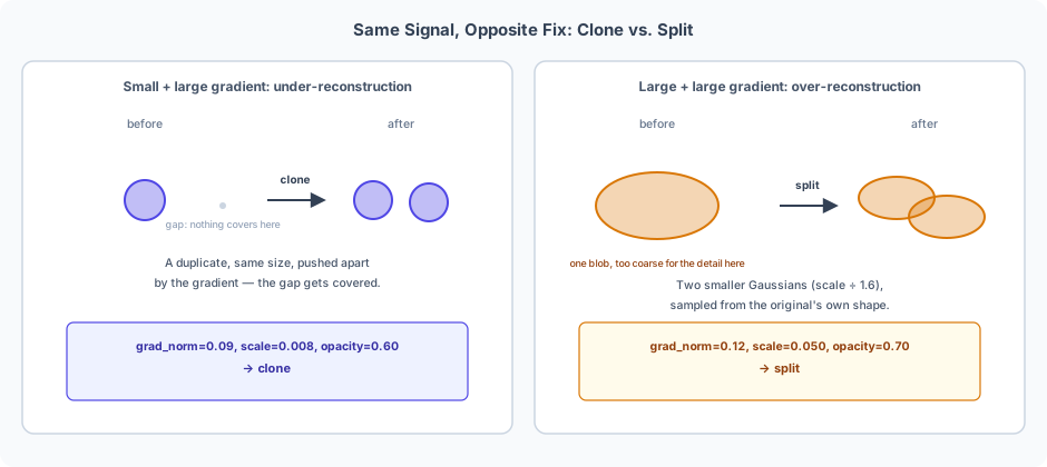
A fixed point cloud from SfM is usually far too sparse to cover a whole scene, so every 100 training iterations the Gaussian set gets grown and pruned based on the view-space positional gradient — how much moving a Gaussian's projected mean would reduce the rendering loss, averaged over those 100 iterations. A gradient above a threshold means a Gaussian is under real pressure to move somewhere it currently isn't fully explaining the photograph, and what happens next depends on its current size:
- Small and under pressure (under-reconstruction): a gap in coverage. Clone the Gaussian — duplicate it in place — and let the gradient on each copy pull them apart to fill the gap.
- Large and under pressure (over-reconstruction): one blob is trying to cover detail it's too coarse to represent. Split it into two smaller Gaussians (scale divided by ), sampled from the original's own shape so the pair starts out already covering roughly the same region, just at finer resolution.
- Opacity below a small threshold: effectively invisible. Prune it outright.
The toy function below uses rounder, more legible numbers than the paper's own threshold purely so the worked table stays readable — the decision logic itself (gradient-vs-threshold, then size-vs-threshold) is unchanged:
def densify_decision(grad_norm, scale, opacity, grad_thresh=0.05, scale_thresh=0.03,
                      opacity_thresh=0.01):
    if opacity < opacity_thresh:
        return "prune"
    if grad_norm > grad_thresh:
        return "split" if scale > scale_thresh else "clone"
    return "keep"

gaussians = [
    dict(grad_norm=0.09, scale=0.008, opacity=0.60),
    dict(grad_norm=0.12, scale=0.050, opacity=0.70),
    dict(grad_norm=0.01, scale=0.020, opacity=0.50),
    dict(grad_norm=0.02, scale=0.010, opacity=0.005),
]
for g in gaussians:
    print(g, "->", densify_decision(**g))
# {'grad_norm': 0.09, 'scale': 0.008, 'opacity': 0.6}  -> clone
# {'grad_norm': 0.12, 'scale': 0.05, 'opacity': 0.7}   -> split
# {'grad_norm': 0.01, 'scale': 0.02, 'opacity': 0.5}   -> keep
# {'grad_norm': 0.02, 'scale': 0.01, 'opacity': 0.005} -> prune
Every 3000 iterations, opacity is also reset to a small value for every surviving Gaussian, which forces any Gaussian that had drifted opaque purely to hide a rendering artifact near the camera (a "floater") to earn its opacity back through the loss — or get pruned next round if it can't.
9. Training Loss, Cost, and What Gaussian Splatting Buys
9.1 The loss
Supervision is photometric only, exactly as NeRF's training section described — render, compare against a real photograph, no depth or point-cloud ground truth anywhere in the objective — with an added structural term:
is plain per-pixel absolute error; is one minus the structural similarity index [6], a patch-level measure of luminance, contrast, and structure agreement that penalizes blur and structural mismatch in a way per-pixel error alone doesn't. Every ordinary gradient step on , , , , and the SH coefficients is interleaved with the densify/split/prune control loop from Section 8.2 — training isn't just optimizing a fixed set of parameters, it's growing and pruning the parameter set itself.
9.2 What the trade actually bought
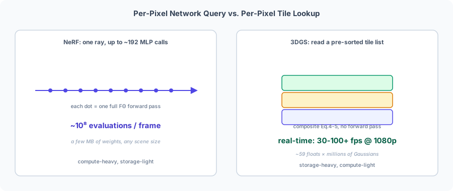
NeRF's own cost section counted roughly MLP forward passes per frame. None of that survives here: rendering a pixel means reading a short, already-sorted list of overlapping splats out of its tile and evaluating Equation (10) and Equation (11) directly — arithmetic on stored numbers, not a network forward pass. That's what makes real-time rendering possible at all: the paper reports 134-154 fps at 1080p on real, complex scenes (higher still, 180-300 fps, on the simpler synthetic Blender scenes) — well clear of the fps bar it sets as the definition of "real-time." The bill doesn't disappear, it moves: a trained scene stores millions of Gaussians, each one roughly floats (mean, quaternion, scale, opacity, degree-3 SH coefficients for RGB), which for a few million Gaussians is easily hundreds of megabytes — against a NeRF MLP's few megabytes of weights, constant regardless of scene complexity. Section 9.2 of the NeRF post called this "the actual subject of the next post," and that's exactly the trade made here: NeRF pays in per-pixel compute for a constant-size, continuously-queryable model; Gaussian Splatting pays in storage for a rasterizable one, and gets the query cost back as almost pure lookup.
10. Putting It Together: A Minimal Reference Implementation
10.1 What this assembles, and what it deliberately leaves out
Everything above is scattered across nine sections, each equation introduced in isolation. This section reassembles the pieces into one small, plain, brute-force renderer covering the forward pass end to end: building a covariance from scale and rotation (Section 3), splatting a Gaussian to screen space (Section 4), evaluating spherical-harmonic color (Section 7), and compositing sorted splats into a pixel (Section 5). Two things are deliberately left out: the tile-based sorting of Section 6, since the whole point there was a performance optimization this code has no reason to reproduce, and the training loop of Sections 8 and 9 — backpropagation and the densify/split/prune control loop are a substantial undertaking of their own, well beyond a single reference snippet. What's left is a plain doubly-nested loop over every pixel and every Gaussian, exactly the cost that Section 6 exists to cut down on — legible over fast, since the goal here is reading the math as code, not shipping a renderer.
10.2 The pipeline
import numpy as np

def quat_to_rotmat(q):
    w, x, y, z = q
    return np.array([
        [1 - 2*(y*y + z*z), 2*(x*y - w*z),     2*(x*z + w*y)],
        [2*(x*y + w*z),     1 - 2*(x*x + z*z), 2*(y*z - w*x)],
        [2*(x*z - w*y),     2*(y*z + w*x),     1 - 2*(x*x + y*y)],
    ])

def build_covariance(log_scale, quat_raw):
    """Section 3.2: the only two quantities gradient descent actually optimizes,
    log_scale and quat_raw, mapped to a valid Sigma on every call."""
    s = np.exp(log_scale)                              # Eq(3): always positive
    q = quat_raw / np.linalg.norm(quat_raw)             # Eq(4): always unit length
    R = quat_to_rotmat(q)
    S = np.diag(s)
    return R @ S @ S.T @ R.T                            # Eq(2)

def project_gaussian(mean, Sigma, W, p_cam, fx, fy, cx, cy):
    """Section 4: one Gaussian's mean and covariance, moved from world space
    into a screen-space mean u and a 2x2 footprint Sigma_2d."""
    t = W @ mean + p_cam                                # Eq(5)
    if t[2] <= 0:
        return None                                     # behind the camera, not visible
    t0, t1, t2 = t
    u = np.array([fx * t0 / t2 + cx, fy * t1 / t2 + cy])  # Eq(6), exact
    J = np.array([
        [fx / t2, 0.0,     -fx * t0 / t2**2],
        [0.0,     fy / t2, -fy * t1 / t2**2],
        [0.0,     0.0,      0.0],
    ])                                                   # Eq(9)
    Sigma_prime = (J @ W @ Sigma @ W.T @ J.T)[:2, :2]     # Eq(7)
    return u, Sigma_prime, t2                             # t2 doubles as the depth sort key

def gaussian_2d(p, u, Sigma_2d):
    """G'(p): Eq(1), restricted to the screen plane, evaluated at pixel p."""
    diff = p - u
    return np.exp(-0.5 * diff @ np.linalg.inv(Sigma_2d) @ diff)

# Section 7: real spherical-harmonic basis, degree 3 (16 terms per channel).
# Constants verified against the reference implementation's utils/sh_utils.py.
SH_C0 = 0.28209479177387814
SH_C1 = 0.4886025119029199
SH_C2 = [1.0925484305920792, -1.0925484305920792, 0.31539156525252005,
         -1.0925484305920792, 0.5462742152960396]
SH_C3 = [-0.5900435899266435, 2.890611442640554, -0.4570457994644658,
         0.3731763325901154, -0.4570457994644658, 1.445305721320277,
         -0.5900435899266435]

def eval_sh(coeffs, d):
    """c(d) for one color channel: Eq(12), all 16 stored k_l^m for l=0..3."""
    x, y, z = d
    xx, yy, zz = x*x, y*y, z*z
    xy, yz, xz = x*y, y*z, x*z
    result = SH_C0 * coeffs[0]
    result += SH_C1 * y * coeffs[1] + SH_C1 * z * coeffs[2] + SH_C1 * x * coeffs[3]
    result += SH_C2[0] * xy * coeffs[4] + SH_C2[1] * yz * coeffs[5]
    result += SH_C2[2] * (2*zz - xx - yy) * coeffs[6]
    result += SH_C2[3] * xz * coeffs[7] + SH_C2[4] * (xx - yy) * coeffs[8]
    result += SH_C3[0] * y * (3*xx - yy) * coeffs[9] + SH_C3[1] * xy * z * coeffs[10]
    result += SH_C3[2] * y * (4*zz - xx - yy) * coeffs[11]
    result += SH_C3[3] * z * (2*zz - 3*xx - 3*yy) * coeffs[12]
    result += SH_C3[4] * x * (4*zz - xx - yy) * coeffs[13]
    result += SH_C3[5] * z * (xx - yy) * coeffs[14] + SH_C3[6] * x * (xx - 3*yy) * coeffs[15]
    return result

def eval_sh_color(sh_coeffs, d):
    """sh_coeffs: (3, 16) array, one row per RGB channel."""
    rgb = np.array([eval_sh(sh_coeffs[c], d) for c in range(3)])
    return np.clip(rgb + 0.5, 0.0, 1.0)                 # matches the reference clamp

def render(gaussians, W, p_cam, fx, fy, cx, cy, width, height, view_dir):
    """Sections 5 and 6.1's math, minus the tiling: every pixel checks every Gaussian."""
    projected = []
    for g in gaussians:
        Sigma = build_covariance(g["log_scale"], g["quat_raw"])
        result = project_gaussian(g["mean"], Sigma, W, p_cam, fx, fy, cx, cy)
        if result is None:
            continue
        u, Sigma_2d, depth = result
        opacity = 1.0 / (1.0 + np.exp(-g["opacity_raw"]))  # raw parameter -> (0,1)
        color = eval_sh_color(g["sh_coeffs"], view_dir)
        projected.append((depth, u, Sigma_2d, opacity, color))

    projected.sort(key=lambda item: item[0])            # front-to-back by depth, Section 6.1

    image = np.zeros((height, width, 3))
    for py in range(height):
        for px in range(width):
            p = np.array([px + 0.5, py + 0.5])          # pixel center
            T = 1.0                                     # accumulated transmittance
            pixel_color = np.zeros(3)
            for depth, u, Sigma_2d, opacity, color in projected:
                alpha = opacity * gaussian_2d(p, u, Sigma_2d)  # Eq(10)
                pixel_color += T * alpha * color                # Eq(11), one term
                T *= (1.0 - alpha)
            image[py, px] = pixel_color
    return image
10.3 A tiny worked scene
Three flat-colored, differently-shaped Gaussians — two round, one an anisotropic ellipse rotated
— in front of an identity-view camera, rendered to a small image and printed as ASCII
brightness so the result is visible without any image-file machinery. Their color coefficients
use only the SH term (a flat color from every direction); eval_sh above still runs its
full 16-term evaluation, it just multiplies 15 of those terms by zero:
def flat_color_coeffs(rgb):
    """A Gaussian with no view-dependence: every SH term above l=0 is zero."""
    sh = np.zeros((3, 16))
    sh[:, 0] = (np.array(rgb) - 0.5) / SH_C0
    return sh

gaussians = [
    dict(mean=np.array([-0.8, 0.0, 3.0]), log_scale=np.log([0.25, 0.25, 0.1]),
         quat_raw=np.array([1.0, 0.0, 0.0, 0.0]), opacity_raw=3.0,
         sh_coeffs=flat_color_coeffs([0.95, 0.95, 0.95])),   # bright, round
    dict(mean=np.array([0.8, 0.0, 3.0]), log_scale=np.log([0.3, 0.3, 0.1]),
         quat_raw=np.array([1.0, 0.0, 0.0, 0.0]), opacity_raw=3.0,
         sh_coeffs=flat_color_coeffs([0.5, 0.5, 0.5])),      # mid-gray, round
    dict(mean=np.array([0.0, 0.6, 3.5]), log_scale=np.log([0.6, 0.2, 0.1]),
         quat_raw=np.array([0.92, 0.0, 0.0, 0.38]), opacity_raw=3.0,
         sh_coeffs=flat_color_coeffs([0.15, 0.15, 0.15])),   # dim, elongated, rotated
]

W, p_cam = np.eye(3), np.zeros(3)
width, height, fx, fy = 50, 22, 45.0, 45.0
image = render(gaussians, W, p_cam, fx, fy, width / 2, height / 2,
                width, height, view_dir=np.array([0.0, 0.0, -1.0]))

ramp = " .:-=+*#%@"
for row in image.mean(axis=2):
    line = "".join(ramp[min(len(ramp) - 1, int(v * (len(ramp) - 1)))] for v in row)
    if line.strip():         # skip the empty margin rows above and below the scene
        print(line.rstrip())
           ....                    ....
         ........                ........
        ..::::::..              ....::....
       ..:------::.            ...::::::...
      ..:-==++==-:..          ...:::--:::...
      .:-=+****+=-:..         ..::------::..
     ..:-=**##**+-:..        ...:---==---:...
     ..:-+*#%%#*+=-:.        ..::--====--::..
     ..:-+*#%%#*+=-:..       ..::--====--::..
     ..:-=**##**+=-:..       ...:---==---:...
      .:-=+****+=-::...       ..::------::..
      ..:-==++==-::....       ...:::--:::...
       ..:------::......       ...::::::...
        ..::::::..........     .....::....
         .........   ......      ........
           ....       ......       ....
                       ......
                        .....
                         ....
The left blob is brighter and rounder than the right, exactly matching the vs. flat colors and equal, isotropic scales assigned to them. The third Gaussian barely registers — dim (), farther away ( against ), and visible only as a faint smear along its own rotated long axis at the bottom edge, exactly the anisotropic, rotated covariance it was built with. Nothing about this image was hand-drawn: every pixel is Section 5's compositing equation, evaluated literally, against Gaussians built exactly as Section 3 describes.
References
- [1]Kerbl, Kopanas, Leimkühler, and Drettakis (2023). 3D Gaussian Splatting for Real-Time Radiance Field Rendering. ACM Transactions on Graphics (SIGGRAPH).
- [2]Zwicker, Pfister, van Baar, and Gross (2001). EWA Volume Splatting. IEEE Visualization (VIS).
- [3]Mildenhall et al. (2020). NeRF: Representing Scenes as Neural Radiance Fields for View Synthesis. European Conference on Computer Vision (ECCV).
- [4]Schönberger and Frahm (2016). Structure-from-Motion Revisited. IEEE Conference on Computer Vision and Pattern Recognition (CVPR).
- [5]Ramamoorthi and Hanrahan (2001). An Efficient Representation for Irradiance Environment Maps. SIGGRAPH.
- [6]Wang, Bovik, Sheikh, and Simoncelli (2004). Image Quality Assessment: From Error Visibility to Structural Similarity. IEEE Transactions on Image Processing.