The Vision Transformer post borrowed one detail from BERT without explaining
it — the [CLS] token, prepended to a sequence purely so the model has one dedicated position to read a
whole-sequence answer back out of. That borrow is a good hint at what BERT actually is: not a new
attention mechanism, not a new module, but the Transformer encoder,
completely unmodified, pointed at a new problem — learning general-purpose language representations from
raw, unlabeled text, before ever being told what downstream task it'll be used for.
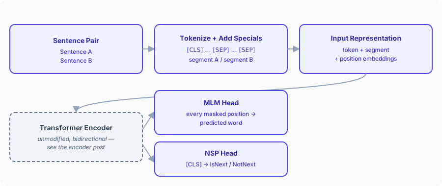
Getting there takes two genuinely new ideas, and this post covers both. First, a bidirectional encoder can't be pretrained the obvious way — predicting a word from a context that already contains that word is a trivial, useless task — so BERT pretrains on a corrupted version of the input instead, called masked language modeling. Second, BERT's input can be a pair of sentences, not just one, which needs a new kind of embedding (segment embeddings) and unlocks a second pretraining task, next sentence prediction. Both ideas, and the fine-tuning step that follows them, are worked through below with the same 6-word toy vocabulary the encoder post used, so there's no new setup to learn before the real content starts.
Contents
- Input Representation — token, segment, and learned positional embeddings for a sentence pair, plus
[CLS]and[SEP] - Masked Language Modeling — why bidirectional pretraining needs corruption, the 80/10/10 rule, and predicting a masked word
- Next Sentence Prediction — a second pretraining task, reading
[CLS]'s output - The Transformer Encoder — the same machinery from the earlier post, completely unmodified and never masked
- Fine-Tuning for Downstream Tasks — adapting one pretrained encoder to different jobs with small, task-specific heads
1. Input Representation
1.1. A sentence pair, not just a sentence
Every post so far in this series has fed the encoder a single sentence. BERT's pretraining tasks need
something richer: a pair of sentences, packed into one sequence, with the model told where one ends and
the other begins. Two special tokens make that possible: [CLS], prepended to the very front of the
sequence — the same role it played for ViT, one dedicated position the model can use to summarize the
whole input — and [SEP], inserted after each sentence to mark its end.
1.2. The toy example
Reusing the encoder post's 6-word vocabulary and its running example sentence as Sentence A, paired with a short new Sentence B:
Sentence A: I think I understand
Sentence B: I love dog
Packed together with the special tokens, that's one 10-token sequence:
[CLS]I think I understand[SEP]I love dog[SEP]
| Position | Token | Segment |
|---|---|---|
| 0 | [CLS] | A |
| 1 | I | A |
| 2 | think | A |
| 3 | I | A |
| 4 | understand | A |
| 5 | [SEP] | A |
| 6 | I | B |
| 7 | love | B |
| 8 | dog | B |
| 9 | [SEP] | B |
Note the trailing [SEP] belongs to Sentence B, not a separate third segment — every token up to and
including the first [SEP] is segment A, everything after it is segment B.
Note: real BERT tokenizes with WordPiece [5], splitting rarer words into subword pieces the same way the encoder post's Token Embeddings note flagged for Transformers generally — "understand" might become "under" + "##stand". This series sticks with whole-word tokens throughout, so the walkthrough below stays focused on what's genuinely new to BERT rather than re-deriving subword splitting.
1.3. Three embeddings, not two
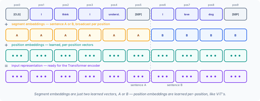
The encoder post's input was token embedding plus positional encoding — two things summed together. BERT's input sums three:
is the familiar lookup from the encoder post's Token Embeddings
module, extended with rows for [CLS]
and [SEP]. is new: exactly two learned vectors, one for "segment A" and one for
"segment B," broadcast identically to every token in that segment — it's what tells the encoder which
sentence a given position came from, since nothing else in the sequence carries that information.
is also new relative to the encoder post specifically: BERT uses a learned positional
embedding table, one trainable vector per position, the same choice ViT made for images
[1] — not the encoder post's fixed sin/cos formula,
Equation (1) and Equation (2).
A useful way to hold the three in your head: token embedding answers "what word," segment embedding answers "whose sentence," and positional embedding answers "which spot." Three independent questions, each with its own small lookup table, summed into one vector that answers all three at once.
1.4. Embeddings as matrix multiplication
The encoder post's Token Embeddings module called embedding lookup "not really computation... closer to 'look up and copy.'" That's true for getting the right numbers by hand, but it's worth seeing the matrix-multiplication form once, since it's the reason these tables can be learned at all — a lookup is just a linear layer whose input happens to be a one-hot vector.
Represent token as a one-hot column vector — length (7, for our tiny vocabulary below), all zeros except a single 1 in the row for — and segment the same way, . Position works slightly differently, covered below; call its selector for now:
Each turns a column into a row, so the shapes work out the same way every other matrix multiplication in this series has: — a single -dimensional embedding row out. That fixes the shapes of the three tables themselves:
| Table | Shape | Rows mean | In our toy example |
|---|---|---|---|
| one per vocabulary word | |||
| one per segment (always exactly 2) | |||
| one per position, up to a fixed cap |
is , 4 here — the same embedding width as every other post in this series. In real BERT, is the big one: a row for every one of tens of thousands of WordPiece pieces, so it holds the large majority of the model's embedding parameters. stays tiny forever — always exactly 2 rows, no matter how long the input gets, since there are always exactly two segments.
's size is worth pausing on, because is not "however long today's sequence happens to be" — it's a fixed hyperparameter, chosen once before pretraining and baked into the table's row count from then on. Real BERT sets . Any input up to 512 tokens draws its position rows from that same fixed table; token 513 has no row to draw from — the table simply doesn't have one, so a longer sequence has to be truncated before it can be encoded at all — nothing in BERT itself splits an over-length input into multiple passes and stitches the results back together; that's an application-level choice (sliding-window chunking, most commonly) you'd have to build around it, not something the architecture does for you. That's the identical constraint the ViT post's Positional Embeddings module hit for image resolution — a learned position table only covers as many positions as it was built with — and exactly what the encoder post's fixed sin/cos formula, Equation (1) and Equation (2), sidesteps entirely: a formula can be evaluated at any position at all, with no table to run out of rows in. Our own toy example never bumps into this, since we only ever built a table exactly as tall as our one 10-token sequence — here, purely because we never needed to be anything bigger.
Worked out for "understand," the 5th row of the 7-row token table below (in the order [CLS], [SEP],
I, think, understand, love, dog):
Every term in that product is except the 1 in the 5th column, which passes "understand"'s row through untouched. is the simplest case of the three: since row of already is position 's embedding, just picks out row directly — there's no separate "position ID" to look up in the first place, unlike tokens and segments.
Note: no real implementation actually builds these one-hot vectors and runs the multiplication — that would mean multiplying a mostly-zero length- vector through the whole table just to recover one row you already knew the address of. Real code (PyTorch's
nn.Embeddingand equivalents) does the obvious thing on the forward pass: index straight into the table,E_tok[t_i]. Equation (2) is a mathematical equivalence, not a description of what runs.It matters anyway because of the gradient. Differentiating with respect to is zero everywhere except row — which is exactly how embedding backprop is implemented: the incoming gradient gets added into that one row, not computed as some dense matrix gradient. The one-hot framing isn't how the forward pass runs; it's why the backward pass is well-defined at all, using the same ordinary backpropagation every other weight matrix in this series already relies on, with no special case carved out for "this particular weight happens to be looked up instead of multiplied densely."
1.5. The embedding table
— reusing the encoder post's table and adding the two new special tokens:
| Token | Embedding |
|---|---|
[CLS] | [0.20, 0.20, 0.20, 0.20] |
[SEP] | [0.10, 0.10, 0.10, 0.10] |
| I | [1, 0, 3, 2] |
| think | [4, 1, 0, 2] |
| understand | [0, 3, 1, 4] |
| love | [2, 2, 4, 0] |
| dog | [3, 0, 2, 1] |
— just two rows, small and hand-picked so they nudge the token embedding without overwhelming it, the same design reasoning the encoder post's Positional Encoding module used. Think of the two rows as colored tags stuck onto every token — amber for "I belong to sentence A," blue for "I belong to sentence B," matching the colors in the figure below:
| Segment | Embedding |
|---|---|
| A | [0.02, 0.02, 0.02, 0.02] |
| B | [-0.02, -0.02, -0.02, -0.02] |
— 10 hand-picked rows, one per position in our sequence:
| Position | Embedding |
|---|---|
| 0 | [0.05, 0.05, 0.05, 0.05] |
| 1 | [0.10, 0.00, 0.00, 0.10] |
| 2 | [0.00, 0.10, 0.10, 0.00] |
| 3 | [0.10, 0.10, 0.00, 0.00] |
| 4 | [0.00, 0.00, 0.10, 0.10] |
| 5 | [0.05, 0.10, 0.05, 0.00] |
| 6 | [0.10, 0.05, 0.00, 0.05] |
| 7 | [0.00, 0.05, 0.10, 0.05] |
| 8 | [0.05, 0.00, 0.05, 0.10] |
| 9 | [0.10, 0.10, 0.10, 0.00] |
1.6. Worked example: position 4 ("understand")
Position 4 is Sentence A's fourth word, "understand" — segment A, position 4:
Three additions, dimension by dimension — the same "no cross-dimension mixing" arithmetic every embedding-sum step in this series has used.
1.7. Result — the full input representation
The identical sum, applied to all ten positions:
| Position | Token | Segment | Input Representation |
|---|---|---|---|
| 0 | [CLS] | A | [0.27, 0.27, 0.27, 0.27] |
| 1 | I | A | [1.12, 0.02, 3.02, 2.12] |
| 2 | think | A | [4.02, 1.12, 0.12, 2.02] |
| 3 | I | A | [1.12, 0.12, 3.02, 2.02] |
| 4 | understand | A | [0.02, 3.02, 1.12, 4.12] |
| 5 | [SEP] | A | [0.17, 0.22, 0.17, 0.12] |
| 6 | I | B | [1.08, 0.03, 2.98, 2.03] |
| 7 | love | B | [1.98, 2.03, 4.08, 0.03] |
| 8 | dog | B | [3.03, -0.02, 2.03, 1.08] |
| 9 | [SEP] | B | [0.18, 0.18, 0.18, 0.08] |
import numpy as np

token_emb = {
    "[CLS]": np.array([0.2, 0.2, 0.2, 0.2]),
    "[SEP]": np.array([0.1, 0.1, 0.1, 0.1]),
    "I": np.array([1, 0, 3, 2], dtype=float),
    "think": np.array([4, 1, 0, 2], dtype=float),
    "understand": np.array([0, 3, 1, 4], dtype=float),
    "love": np.array([2, 2, 4, 0], dtype=float),
    "dog": np.array([3, 0, 2, 1], dtype=float),
}

tokens = ["[CLS]", "I", "think", "I", "understand", "[SEP]", "I", "love", "dog", "[SEP]"]
segments = [0, 0, 0, 0, 0, 0, 1, 1, 1, 1]
seg_emb = {0: np.array([0.02, 0.02, 0.02, 0.02]), 1: np.array([-0.02, -0.02, -0.02, -0.02])}

pos_emb = np.array([
    [0.05, 0.05, 0.05, 0.05],
    [0.10, 0.00, 0.00, 0.10],
    [0.00, 0.10, 0.10, 0.00],
    [0.10, 0.10, 0.00, 0.00],
    [0.00, 0.00, 0.10, 0.10],
    [0.05, 0.10, 0.05, 0.00],
    [0.10, 0.05, 0.00, 0.05],
    [0.00, 0.05, 0.10, 0.05],
    [0.05, 0.00, 0.05, 0.10],
    [0.10, 0.10, 0.10, 0.00],
])

input_repr = np.array([
    token_emb[tok] + seg_emb[seg] + pos_emb[i]
    for i, (tok, seg) in enumerate(zip(tokens, segments))
])
print(np.round(input_repr, 2))
# [[0.27 0.27 0.27 0.27]
#  [1.12 0.02 3.02 2.12]
#  [4.02 1.12 0.12 2.02]
#  [1.12 0.12 3.02 2.02]
#  [0.02 3.02 1.12 4.12]
#  [0.17 0.22 0.17 0.12]
#  [1.08 0.03 2.98 2.03]
#  [1.98 2.03 4.08 0.03]
#  [3.03 -0.02 2.03 1.08]
#  [0.18 0.18 0.18 0.08]]
This 10x4 matrix is what feeds into the Transformer encoder — same shape of thing as every other post in this series has produced by the end of its own input-construction module, just with one more embedding folded in and twice as many rows, since there are now two sentences instead of one.
1.8. Up next: masked language modeling
With a sentence pair encoded, the natural next question is what BERT is actually trained to predict. Unlike the decoder post's next-word objective, which falls out naturally from reading left to right, bidirectional pretraining needs its own, less obvious trick — covered next.
2. Masked Language Modeling
2.1. Why bidirectional pretraining isn't as simple as it sounds
The decoder post trained on a task that's easy to state: predict the next word, given only the words before it. That works specifically because the causal mask — Equation (8) — makes it impossible for the model to see the answer; token 's prediction is computed from a representation that provably never had access to token or anything after it.
BERT's encoder has no causal mask at all — every position can attend to every other position, in both directions, from the very first layer. That's exactly what makes it good at building rich, context-aware representations. But it also means the obvious pretraining task — "predict word , using the whole sentence as context" — is trivial to the point of uselessness: word 's own embedding is already sitting right there in the input at position . Self-attention can satisfy that "prediction" by doing nothing more than copying the value straight through, at every layer, without learning anything about context at all.
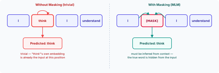
BERT's fix, from the original paper [1]: don't show the model the real word at every position. Corrupt a fraction of the input first, and only ask it to predict the corrupted positions. With the answer no longer present in the input, the only way to recover it is to actually use the surrounding context — which is the whole point.
If that sounds familiar, it should — it's a machine-scale version of the Cloze test, a language-class
exercise where a word is blanked out of a passage and a student has to fill it in using only the sentences
around it. A student can't just read the answer off the page; the blank forces her to actually understand
the passage. [MASK] is BERT's blank, and predicting it — this module's whole job — is that same exercise,
run over billions of blanked-out words instead of one classroom worksheet.
2.2. The 80/10/10 rule
15% of a training sequence's positions are chosen to be predicted. What the model actually sees at each
chosen position, though, isn't always [MASK]:
| Case | Probability | Fed to the model at that position | Label used in the loss |
|---|---|---|---|
| Mask | 80% | [MASK] | the original word |
| Random | 10% | a random word from the vocabulary | the original word |
| Unchanged | 10% | the original word, untouched | the original word |
All three cases are scored identically — the model always has to predict the true original word at that
position. Only what's fed in changes. The 10%/10% cases exist for a subtle but important reason: if
[MASK] were the only kind of corruption, the model could learn a shortcut — "only build a careful
representation when I see the literal [MASK] token, and coast otherwise" — but [MASK] only ever
appears during pretraining, never at fine-tuning time (covered later, in Fine-Tuning for Downstream
Tasks). Occasionally corrupting a position without using
[MASK] at all forces the model to keep building good representations for every token, not just the
visibly-corrupted ones, closing that gap between how it's pretrained and how it's actually used later.
2.3. Worked example: masking "understand"
Take position 4 from the Input Representation module — "understand," segment A — as the position chosen
for the 80% [MASK] case. Its token embedding is swapped for [MASK]'s, a hand-picked vector like
[CLS] and [SEP] got in that same module:
Note:
[MASK]belongs in exactly the way[CLS]and[SEP]do — a genuine vocabulary entry with its own input embedding, an 8th row alongside the 7 shown in the Input Representation module's token table. It's introduced here instead of there purely because it wasn't needed until now, not because it's a different kind of thing. That's the input side, though — the output side (the softmax a few steps below, which predicts what word was hidden) draws from a deliberately smaller, separate list: I, think, understand, love, dog, cat, excluding[MASK],[CLS], and[SEP], since none of those could ever be the correct answer to "what word was masked here." Real BERT actually ties its output weights to the entire input vocabulary, specials included, via weight sharing with — so nothing architecturally stops it from assigning[MASK]some probability as an answer, it just never has a reason to, since training labels are never[MASK]itself.
Running the same sum as the Input Representation module — Equation (1) — with [MASK] in place of "understand" at
position 4, segment A, position embedding unchanged:
Every other position keeps the exact values from the Input Representation module's result table — only position 4 changes.
masked_tokens = list(tokens)
masked_tokens[4] = "[MASK]"
token_emb["[MASK]"] = np.array([0.3, 0.3, 0.3, 0.3])

masked_input_repr = np.array([
    token_emb[tok] + seg_emb[seg] + pos_emb[i]
    for i, (tok, seg) in enumerate(zip(masked_tokens, segments))
])
print(np.round(masked_input_repr[4], 2))
# [0.32 0.32 0.42 0.42]
2.4. The output layer: from masked position to predicted word
Running this masked sequence through the full encoder isn't repeated here — it's exactly the Transformer Encoder module's computation, unmodified, on this input instead. So, like the ViT post's classification head module, this step starts from a clearly-labeled hypothetical: suppose that after passing through the encoder, position 4's final output vector is
A linear projection back up to vocabulary size, then softmax — the identical shape of computation as the decoder post's output layer, Equation (2), just reading off one masked position instead of every position at once:
is here, one column per word in our toy vocabulary (real BERT predicts over its full WordPiece vocabulary, tens of thousands of subword pieces wide):
| I | think | understand | love | dog | cat | |
|---|---|---|---|---|---|---|
| logits | -0.110 | 0.460 | 0.120 | 0.050 | 0.250 | -0.270 |
| softmax probability | 0.134 | 0.236 | 0.168 | 0.157 | 0.191 | 0.114 |
def softmax(x, axis=-1):
    x = x - np.max(x, axis=axis, keepdims=True)
    e = np.exp(x)
    return e / np.sum(e, axis=axis, keepdims=True)

vocab = ["I", "think", "understand", "love", "dog", "cat"]
h_mask = np.array([0.1, 0.6, 0.2, 0.9])

W_vocab = np.array([
    [0.2, 0.1, -0.3, 0.4, -0.1, 0.2],
    [-0.1, 0.3, 0.2, -0.2, 0.4, -0.3],
    [0.3, -0.2, 0.1, 0.2, -0.3, 0.1],
    [-0.2, 0.4, -0.1, 0.1, 0.2, -0.2],
])
b_vocab = np.array([0.05, -0.05, 0.1, 0.0, -0.1, 0.05])

logits = h_mask @ W_vocab + b_vocab
probs = softmax(logits)
print(np.round(logits, 3))
# [-0.11  0.46  0.12  0.05  0.25 -0.27]
print(np.round(probs, 3))
# [0.134 0.236 0.168 0.157 0.191 0.114]
print(vocab[np.argmax(probs)])
# think
The top prediction is "think," not "understand" — a miss, and an expected one: exactly like the decoder post's greedy-decoding example, and here are hand-picked stand-ins, not the product of training. What this worked example demonstrates is purely the mechanism: any encoder output vector at a masked position deterministically becomes a full probability distribution over the vocabulary, and training's whole job is nudging that distribution — over millions of masked positions — toward putting the true word on top.
2.5. Up next: next sentence prediction
Masked language modeling teaches the encoder to build good token-level representations from bidirectional
context. It says nothing, though, about the relationship between the two sentences packed into the
input — that's what [SEP] and segment embeddings were introduced for in Input Representation, and it's
the subject of BERT's second pretraining task, next.
3. Next Sentence Prediction
3.1. A sentence-pair-level task
Masked language modeling operates purely at the token level — one prediction per masked position. Next
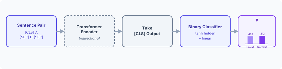
sentence prediction (NSP) is different: one prediction for the entire pair, using exactly the mechanism
the ViT post's classification head established — read [CLS]'s final output,
run it through a small classifier.
The task itself: given Sentence A and Sentence B as packed in Input Representation, decide whether B genuinely follows A in the original text (label IsNext) or was swapped in from somewhere unrelated (label NotNext). It's a machine-scale version of a familiar reading-comprehension question: do these two sentences continue naturally into each other, or do they read like they were yanked from two different books? Half of BERT's pretraining pairs are constructed each way, so the classifier has a real, balanced signal to learn from.
3.2. The formula
Structurally identical to Equation (5), ViT's classification head — a hidden layer with , a linear layer down to the number of classes (2, this time), then softmax:
3.3. Worked example
Same hypothetical-vector approach as the MLM head above: suppose that after passing through the encoder,
[CLS]'s final output (position 0) is
is ; :
is — two classes, IsNext and NotNext; :
| IsNext | NotNext | |
|---|---|---|
| logits | 0.060 | 0.106 |
| softmax probability | 0.488 | 0.512 |
h_cls = np.array([0.5, 0.3, 0.7, 0.2])

W1 = np.array([
    [0.2, 0.1, -0.1, 0.3],
    [0.1, -0.2, 0.3, 0.1],
    [-0.1, 0.3, 0.2, -0.2],
    [0.3, 0.1, -0.2, 0.2],
])
b1 = np.array([0.0, 0.0, 0.0, 0.0])

W2 = np.array([
    [0.6, -0.3],
    [-0.2, 0.5],
    [0.4, -0.1],
    [-0.3, 0.6],
])
b2 = np.array([0.0, 0.0])

hidden = np.tanh(h_cls @ W1 + b1)
logits = hidden @ W2 + b2
probs = softmax(logits)

print(np.round(hidden, 3))
# [0.119 0.217 0.139 0.08 ]
print(np.round(probs, 3))
# [0.488 0.512]   # IsNext, NotNext
NotNext edges out IsNext, 0.512 to 0.488 — as close to a coin flip as the MLM head's result above, for the
same reason: hand-picked weights and a made-up h_cls have no reason to produce a confident answer. In a
trained model, this same head — read [CLS], run the classifier — is what tells you whether two sentences
actually belong together.
3.4. Pretraining is both tasks at once
BERT isn't trained on MLM, then NSP — every training batch computes both losses on the same forward pass through the same encoder, and adds them together:
only touches the masked positions; only touches
[CLS]. Nothing about the encoder itself is task-specific — the same bidirectional self-attention,
running once, produces representations that both heads read from.
"The masked positions," plural, is doing real work in that sentence — MLM doesn't mask and predict one word, run the encoder again, mask a different word, and repeat. ~15% of a sequence's positions are chosen as one set, all at once, and every one of them is predicted from the same single forward pass:
is that set of masked positions (position 4 alone, in our worked example — a real sequence would have
several); is the corrupted sequence actually fed to the encoder, masked_input_repr after it's
been run through the Transformer Encoder module; is the true original word at position , the
label. Equation (8) is exactly the term for one — the worked example
above computed it by hand for alone, but the same , , and
softmax apply independently at every other too, all reading off the one encoder pass that
already computed a representation for every position, masked or not. Summing (rather than, say, averaging)
those per-position log-probabilities is what makes a sequence with more masked positions contribute a
proportionally larger loss.
Concretely, for : is the fixed, known label "understand," so the term the sum actually adds is — whatever probability the softmax in Equation (8) happened to assign to that specific word. In the worked numbers there, that's the third entry of the distribution, , giving . Notice this has nothing to do with which word the model ranked highest — "think" got the top spot at , but the loss doesn't look at rankings at all, only at how much probability landed on the one word that was actually correct.
Note: it's easy to get the direction backwards here. Loss is minimized during training — lower is better — and its floor really is 0, but that floor is reached when : the model putting (near-)certain probability on the correct word, so . isn't the good case, and it isn't 0 either — it's . That happens if the model instead assigns the correct label probability 0, giving : the worst possible loss, not the best. Cross-entropy is shaped this way on purpose — uncertainty costs a little, confidently wrong costs an unbounded amount, confidently right costs nothing — and every formula in this post, including the fine-tuning losses in module 5, behaves the same way.
Note: NSP's usefulness turned out to be more limited than the original paper assumed. RoBERTa [4] later found that dropping NSP entirely and training on longer, contiguous spans of text instead matched or beat BERT's original results — evidence that most of BERT's power comes from masked language modeling on the encoder itself, not from the sentence-pair task layered on top of it. NSP is kept in this post because it's what motivated segment embeddings and the
[SEP]-separated sentence-pair input in the first place, both of which later encoder models generally kept even after dropping NSP.
3.5. Up next: the Transformer encoder
Both pretraining heads read from the same place — the encoder's output — and neither one has touched the encoder itself yet. That's next: confirming, explicitly, that nothing about self-attention had to change to make any of this work.
4. The Transformer Encoder
4.1. Reused, unmodified, and never masked
Every module so far has referred to "the encoder's output" without recomputing it — deliberately, because
there's nothing new to compute. input_repr (from Input Representation) or masked_input_repr (from
Masked Language Modeling) is a legal input
to The Transformer Encoder exactly as originally written: Q/K/V
projection, self-attention (Equation (7)), multi-head attention, the feed-forward network,
and the residual-plus-normalization wrapper around each sub-layer — all of it unchanged, the same reuse
the ViT post already demonstrated for images.
One thing is worth stating plainly rather than leaving implicit, though, since Masked Language Modeling leaned on it directly: BERT's self-attention is never causally masked. The encoder post introduced the causal mask — Equation (8) and Equation (9) — as something a decoder-style model needs, and the decoder post confirmed it's not optional there. BERT sits at the opposite extreme: every position attends to every other position, left and right, in every layer, always. That's precisely the property that made Masked Language Modeling's masking trick necessary in the first place — an encoder that could see the future the way a decoder can't is exactly what makes naively predicting a word from its own unmodified context trivial.
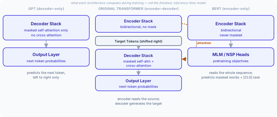
Three architectures, one shared vocabulary of parts: GPT [3] keeps the decoder stack and drops the encoder and cross-attention entirely, predicting strictly left to right. The original Transformer keeps both, connected by cross-attention, for sequence-to-sequence tasks like translation. BERT keeps only the encoder, drops masking entirely, and swaps the output layer for pretraining heads that get discarded once pretraining is done — which is exactly where fine-tuning picks up.
This is what each architecture computes during training — the original Transformer's middle column, in
particular, is the teacher-forcing view the decoder post's output layer module
described, a full target sequence fed in at once rather than the one-token-at-a-time loop actual generation
uses. BERT's column is narrower still: it's specifically pretraining, not training in general — those
MLM/NSP heads exist only to shape the encoder's weights and are gone by the time anyone actually uses the
model. The inference-time picture for a deployed, fine-tuned BERT looks like Figure 6 below instead:
Encoder Stack → task-specific head → task output, with no MLM or NSP anywhere in it.
4.2. Up next: fine-tuning
Pretraining produces one encoder that's good at building context-aware representations, plus two heads that are useful only for the pretraining tasks themselves and nothing else. The last module covers what actually happens to that encoder afterward: reusing it, largely unchanged, for real downstream tasks.
5. Fine-Tuning for Downstream Tasks
5.1. One encoder, several small heads
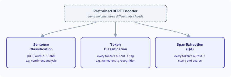
MLM and NSP exist purely to shape the encoder's weights during pretraining — by the time pretraining is done, both of their heads are thrown away. What's kept is the encoder itself: a stack of blocks that has learned, from a large amount of unlabeled text, how to turn a token sequence into context-aware vectors. Fine-tuning takes that pretrained encoder, keeps its weights (as a starting point, further updated during fine-tuning rather than frozen), and attaches a new, small, task-specific head in place of MLM/NSP's — the same "swap the last piece, reuse everything before it" pattern the ViT post's classification head already used, just with the choice of which position(s) to read now depending on the task:
| Task type | Example | Reads |
|---|---|---|
| Sequence classification | sentiment analysis | [CLS]'s output |
| Sequence-pair classification | does sentence B follow from sentence A | [CLS]'s output — literally NSP's own head shape, retrained on a real task |
| Token classification | named entity recognition | every token's own output |
| Span extraction | question answering | every token's output, scored for "start of answer" and "end of answer" |
5.2. Loss functions for each task
The encoder doesn't care what task it's being fine-tuned for — but the loss does, since it has to match the shape of whatever's being predicted. All four below are cross-entropy in spirit, the same log-loss Equation (13) already used for MLM, just pointed at different targets.
Sequence (and sequence-pair) classification — a single softmax over classes, read from
[CLS], penalizing the negative log-probability the model assigned to the true label :
This is Equation (9) (NSP) exactly, with . Any sequence-level task — sentiment, natural
language inference, spam detection — is the identical formula; only and the training data change.
Sequence-pair classification uses this same head unmodified too, since the "pair" is entirely handled at
the input side (two segments packed with [SEP], back in Input Representation) — the loss has no idea, and
no need to know, whether [CLS]'s representation came from one sentence or two.
Token classification — one prediction per position instead of one per sequence, so the loss sums a per-token cross-entropy across every labeled position:
Compare this to Equation (13), MLM's own loss — same "sum of per-position log-probabilities"
shape, but the sum now runs over every real token (real implementations exclude [CLS], [SEP], and
padding positions from it), not just a masked 15%, and each is a tag — person, location,
organization, other — rather than a hidden word being reconstructed.
Span extraction (QA) is the least obvious of the four, since there's no per-token label at all — only one correct start position and one correct end position for the whole sequence. Two learned vectors, and , each score every position by a dot product with its output vector — for the start score, for the end score — and a softmax over all positions turns those scores into two distributions, and : "where does the answer start," "where does it end." The loss is the sum of both correct positions' negative log-likelihoods (some implementations average instead):
The nuance worth sitting with here: span extraction is not "classify every token as start-of-answer or not" — that would be per-token binary classification, structurally identical to Equation (15) with . It's a single -way choice for the start and a separate -way choice for the end, so what's being predicted from is "which position in this specific sequence," not a fixed label vocabulary at all — the "vocabulary" is literally the sequence length, and it's different for every example.
Designing a new fine-tuning task, in practice, is choosing which of these four shapes actually fits — which vector(s) to read, and what the label space looks like — not inventing new machinery. The encoder, and the general softmax-plus-cross-entropy recipe underneath all four losses, stay exactly the same.
Every one of the four losses above is reading from a vector produced the same way: a linear-layer-plus-
softmax, either on [CLS] alone or on every position the way the decoder post's output
layer already did, Equation (2) — nothing new to
the mechanism itself, only to which position(s) get read and what the labels mean. Figure 6 puts the three
per-task shapes side by side:
None of this needs new arithmetic worked through by hand — every projection here is the identical shape
of computation this series has built up across four posts: a linear layer, sometimes a nonlinearity,
sometimes a softmax, reading from either [CLS] or every position, depending on what the task actually
asks for. What's genuinely new about fine-tuning isn't the mechanism; it's that the encoder no longer
starts from random weights. It starts already knowing, from pretraining, a great deal about how language
fits together — and fine-tuning only has to teach it the comparatively small remaining step: which of
those learned patterns actually matter for one specific task.
That completes the trip from a bare Transformer encoder to BERT: a sentence-pair input representation
built from three summed embeddings, masked language modeling as the trick that makes bidirectional
pretraining possible at all, next sentence prediction reading [CLS] for a sentence-pair-level signal,
an entirely unmodified and never-masked encoder underneath both, and a fine-tuning step that swaps out
the pretraining heads for whatever a downstream task actually needs. Every later encoder-only model —
RoBERTa, ELECTRA, and the rest — is a variation on exactly this recipe, not a departure from it.
References
- [1]Devlin et al. (2018). BERT: Pre-training of Deep Bidirectional Transformers for Language Understanding. Conference of the North American Chapter of the Association for Computational Linguistics: Human Language Technologies (NAACL-HLT).
- [2]Vaswani et al. (2017). Attention Is All You Need. Conference on Neural Information Processing Systems (NeurIPS).
- [3]Radford et al. (2018). Improving Language Understanding by Generative Pre-Training. OpenAI.
- [4]Liu et al. (2019). RoBERTa: A Robustly Optimized BERT Pretraining Approach.
- [5]Wu et al. (2016). Google's Neural Machine Translation System: Bridging the Gap between Human and Machine Translation.