The Transformer is the backbone of most modern language and vision models. But papers and lecture slides tend to stack several matrix operations on top of each other, which makes it hard to see exactly what each module takes in and what it hands off to the next one.
This post is the first entry in a series that takes the Transformer apart one module at a time, starting with the encoder half. Instead of the tens-of-thousands-dimensional vectors used in real models, we track a tiny example — 4 tokens with 4-dimensional embeddings — all the way through by hand. The numbers are kept simple enough that you don't need a calculator; just follow the tables with your eyes. Each step also comes with a short, runnable Python snippet so you can reproduce the numbers yourself.
Contents
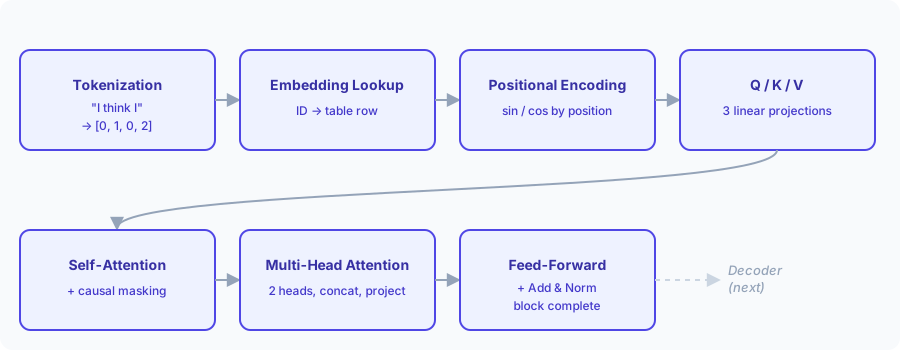
This post covers the encoder half of the Transformer:
- Token embeddings — turning words into vectors
- Positional encoding — adding order information
- Query, Key, Value — three ways of looking at the same vector
- Self-attention — letting words look at each other, plus causal masking
- Multi-head attention — running several attention heads in parallel
- Feed-forward network — residual connections, layer normalization, and assembling a full encoder block
The decoder — cross-attention and generating output — is covered in a follow-up post.
1. Token Embeddings
1.1. Why embeddings are needed
Neural networks only work with numbers. You can't feed a string like "I" or "think" directly into a matrix multiplication, so the first step in a Transformer is always to turn text into numeric vectors. Those vectors are called embeddings.
The process has two parts:
- Tokenization — split the sentence into words (tokens) and assign each one an integer ID.
- Embedding lookup — pull the row that matches that ID out of a pre-trained table (the embedding table).
Neither step is really "computation" — it's closer to "look up and copy." Actual arithmetic doesn't show up until the next module, positional encoding.
1.2. Example sentence
We'll use this 4-word sentence throughout:
I think I understand
Notice "I" shows up twice, at the first and third positions. That's on purpose — it'll let us see, later in this post, exactly what positional encoding adds that a plain embedding lookup can't.
1.3. Step 1 — Tokenization
Split the sentence into words and look up each word's ID in a vocabulary. Our toy vocabulary has just 6 words (real models typically use 30,000-100,000):
| ID | Word |
|---|---|
| 0 | I |
| 1 | think |
| 2 | understand |
| 3 | love |
| 4 | dog |
| 5 | cat |
Running "I think I understand" through the vocabulary gives:
| Position | Word | ID |
|---|---|---|
| 1 | I | 0 |
| 2 | think | 1 |
| 3 | I | 0 |
| 4 | understand | 2 |
Positions 1 and 3 both map to ID 0 — same word, same ID, so far no difference at all.
vocab = {"I": 0, "think": 1, "understand": 2, "love": 3, "dog": 4, "cat": 5}
sentence = ["I", "think", "I", "understand"]

token_ids = [vocab[word] for word in sentence]
print(token_ids)
# [0, 1, 0, 2]
1.4. Step 2 — The embedding table
Each word in the vocabulary is paired with a pre-trained 4-dimensional vector. The whole table is called the embedding table. (Real models use 768, 1024, or more dimensions — we shrink it to 4 so it fits on screen.)
| ID | Word | Embedding Vector |
|---|---|---|
| 0 | I | [1, 0, 3, 2] |
| 1 | think | [4, 1, 0, 2] |
| 2 | understand | [0, 3, 1, 4] |
| 3 | love | [2, 2, 4, 0] |
| 4 | dog | [3, 0, 2, 1] |
| 5 | cat | [1, 4, 0, 3] |
These values are the result of training. For this example, assume training is already done and just use the fixed values above.
1.5. Step 3 — Lookup: pulling out the matching rows
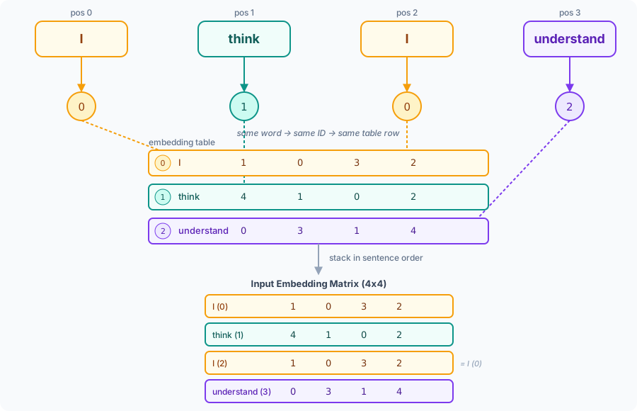
Our sentence's IDs were [0, 1, 0, 2]. All we do is pull the matching row out of the embedding table for each ID, in order. No multiplication, no addition.
- ID 0 (I) → grab row
[1, 0, 3, 2] - ID 1 (think) → grab row
[4, 1, 0, 2] - ID 0 (I) → grab row
[1, 0, 3, 2]— the exact same row as the first one - ID 2 (understand) → grab row
[0, 3, 1, 4]
import numpy as np

embedding_table = np.array([
    [1, 0, 3, 2],  # I
    [4, 1, 0, 2],  # think
    [0, 3, 1, 4],  # understand
    [2, 2, 4, 0],  # love
    [3, 0, 2, 1],  # dog
    [1, 4, 0, 3],  # cat
])

input_embeddings = embedding_table[token_ids]
print(input_embeddings)
# [[1 0 3 2]
#  [4 1 0 2]
#  [1 0 3 2]
#  [0 3 1 4]]
1.6. Result — the input embedding matrix
Stacking the four rows in sentence order gives the 4x4 matrix the Transformer actually receives as input:
| Word | Embedding Vector |
|---|---|
| I | [1, 0, 3, 2] |
| think | [4, 1, 0, 2] |
| I | [1, 0, 3, 2] |
| understand | [0, 3, 1, 4] |
Each row is a word, and each word is represented by its own 4-dimensional vector. Rows 1 and 3 are identical — both are "I," and the embedding table has no way of knowing which "I" is which. This matrix carries no information about word order at all. Adding that order information is the job of the next module: positional encoding.
Note: real Transformers go one step further and split words into subword tokens — "playing" might become "play" + "##ing". This series sticks with whole-word tokens to keep the concept clear.
2. Positional Encoding
2.1. Why position matters
The embedding matrix from module 1 treats the sentence as a bag of words — nothing in it says which word came first, and as we just saw, two occurrences of the same word ("I" at position 1 and position 3) produce the exact same vector. The Transformer needs some way to inject "this is word number 0, this is word number 1, ..." into the vectors themselves.
The classic solution (from the original "Attention Is All You Need" paper [1]) is to compute a fixed positional encoding vector for each position and add it directly to the token embedding. No learning involved — it's just a formula.
2.2. The formula
For position and dimension index in a -dimensional embedding, the even and odd dimensions each follow their own formula. is just the size of the embedding vector — the same number of dimensions we picked for the token embeddings in module 1 (4, in our example), since the positional encoding has to be added to the token embedding dimension-by-dimension:
Each dimension in Equation (1) and Equation (2) is a sine or cosine wave with a different frequency, so every position ends up with a unique, bounded ( to ) fingerprint — regardless of which word happens to sit there.
2.3. Step 1 — Compute the positional encoding table
With (matching the embedding size from module 1) and 4 positions (matching our 4-token sentence), plugging Equation (1) and Equation (2) in gives:
| Position | Positional Encoding Vector |
|---|---|
| 0 | [0.00, 1.00, 0.00, 1.00] |
| 1 | [0.84, 0.54, 0.01, 1.00] |
| 2 | [0.91, -0.42, 0.02, 1.00] |
| 3 | [0.14, -0.99, 0.03, 1.00] |
(odd dimensions — 1 and 3 — come from ; even dimensions — 2 and 4 — come from )
You don't need to compute sine and cosine by hand — just read the table. The code below reproduces it exactly:
import numpy as np

def positional_encoding(seq_len, d_model):
    positions = np.arange(seq_len)[:, None]           # shape (seq_len, 1)
    dims = np.arange(d_model)[None, :]                 # shape (1, d_model)
    angle_rates = 1 / np.power(10000, (2 * (dims // 2)) / d_model)
    angles = positions * angle_rates
    pe = np.zeros((seq_len, d_model))
    pe[:, 0::2] = np.sin(angles[:, 0::2])
    pe[:, 1::2] = np.cos(angles[:, 1::2])
    return pe

pe = positional_encoding(seq_len=4, d_model=4)
print(np.round(pe, 2))
# [[ 0.    1.    0.    1.  ]
#  [ 0.84  0.54  0.01  1.  ]
#  [ 0.91 -0.42  0.02  1.  ]
#  [ 0.14 -0.99  0.03  1.  ]]
2.4. Step 2 — Add it to the token embeddings
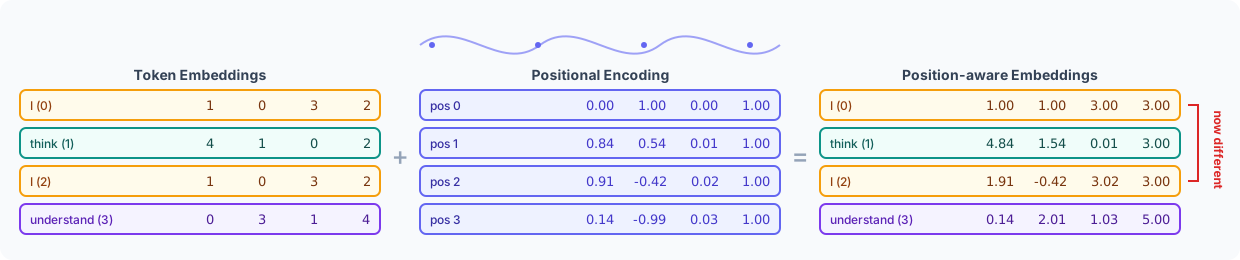
The final step is plain element-wise addition: token embedding + positional encoding, dimension by dimension.
| Word (pos) | Token Embedding | + Positional Encoding | = Position-aware Embedding |
|---|---|---|---|
| I (0) | [1, 0, 3, 2] | [0.00, 1.00, 0.00, 1.00] | [1.00, 1.00, 3.00, 3.00] |
| think (1) | [4, 1, 0, 2] | [0.84, 0.54, 0.01, 1.00] | [4.84, 1.54, 0.01, 3.00] |
| I (2) | [1, 0, 3, 2] | [0.91, -0.42, 0.02, 1.00] | [1.91, -0.42, 3.02, 3.00] |
| understand (3) | [0, 3, 1, 4] | [0.14, -0.99, 0.03, 1.00] | [0.14, 2.01, 1.03, 5.00] |
Each entry adds up dimension by dimension — first value with first value, second with second, and so on — but it's the same vector doing the traveling through the pipeline, not four independent numbers.
position_aware_embeddings = input_embeddings + pe
print(np.round(position_aware_embeddings, 2))
# [[1.   1.   3.   3.  ]
#  [4.84 1.54 0.01 3.  ]
#  [1.91 -0.42 3.02 3.  ]
#  [0.14 2.01 1.03 5.  ]]
2.5. Result — the position-aware embedding matrix
| Word | Position-aware Embedding Vector |
|---|---|
| I | [1.00, 1.00, 3.00, 3.00] |
| think | [4.84, 1.54, 0.01, 3.00] |
| I | [1.91, -0.42, 3.02, 3.00] |
| understand | [0.14, 2.01, 1.03, 5.00] |
This is the matrix that actually flows into the first attention layer. Compare row 1 and row 3 — both started out as the exact same "I" vector, [1, 0, 3, 2], in module 1. Now they're different: [1.00, 1.00, 3.00, 3.00] versus [1.91, -0.42, 3.02, 3.00]. Nothing about the word changed — only its position did, and that alone was enough to pull the two vectors apart. This is precisely what positional encoding is for.
Note: because the positional values are bounded between -1 and 1, they nudge the embedding rather than overwhelm it. That's a deliberate design choice — a positional signal made of huge numbers would drown out the meaning captured by the token embedding.
3. Query, Key, and Value
3.1. Why three different vectors?
The next module in the series, self-attention, lets every token gather information from the other tokens in the sentence — but weighted by relevance. Before that comparison can happen, each token's position-aware embedding is projected into three separate role-specific vectors:
- Query (Q) — what this token is looking for in other tokens
- Key (K) — what this token has to offer, as a label other tokens can match against
- Value (V) — the actual content this token hands over if it turns out to be relevant
A library catalog is a decent analogy for this blog in particular. Say you walk up to the card catalog looking for something:
- Your search topic is the Query — "I'm looking for something about space travel."
- Each book's index card lists subject keywords — that's the Key — "this book is about: rockets, astronauts, moon landing."
- The book itself, the thing you actually walk away with once a card matches your topic, is the Value.
The important part: matching happens between Query and Key, but what gets returned is the Value. You don't take the index card home — you take the book. The next module (self-attention) is exactly this: compare every token's Query against every other token's Key to get a relevance score, then use those scores to blend together the Values.
3.2. How they are computed
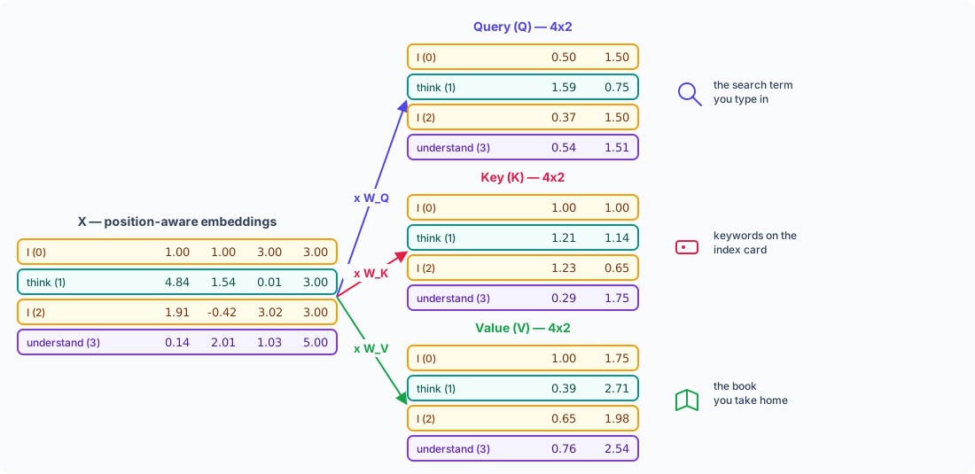
Q, K, and V are each a separate linear projection of the same input — the position-aware embedding matrix from module 2 — using three separate weight matrices:
In a real model, , , and in Equation (3) are learned during training and have shape , where is often smaller than (the multi-head module later on explains why). Here we project our 4-dimensional embeddings down to 2-dimensional Q, K, and V vectors, using small hand-picked weights so you can see exactly which input dimensions feed each output dimension.
3.3. Example weight matrices
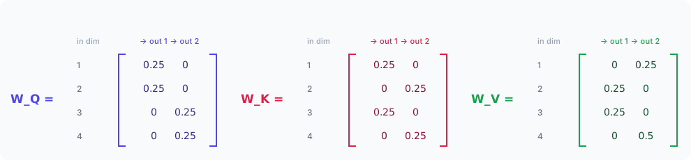
Three different ways of mixing the same four numbers — which is exactly why Q, K, and V end up as three different vectors for the same token.
Note: in a trained model these weights are floating-point numbers learned by backpropagation, not hand-picked ones. We keep them small here on purpose — with larger weights, the dot products in the self-attention step below get large enough that the softmax turns into a near-coin-flip winner-take-all, which would hide the "blend of everything" behavior we're trying to see.
3.4. Step — Project each token into Q, K, V
Worked example for "I" at position 0, whose position-aware embedding (from module 2) is [1.00, 1.00, 3.00, 3.00]:
The same projection, applied to all four tokens:
| Word (pos) | Query (Q) | Key (K) | Value (V) |
|---|---|---|---|
| I (0) | [0.50, 1.50] | [1.00, 1.00] | [1.00, 1.75] |
| think (1) | [1.59, 0.75] | [1.21, 1.14] | [0.39, 2.71] |
| I (2) | [0.37, 1.50] | [1.23, 0.65] | [0.65, 1.98] |
| understand (3) | [0.54, 1.51] | [0.29, 1.75] | [0.76, 2.54] |
Notice the two "I" rows (position 0 and position 2) now have different Q, K, and V vectors, even though they came from the same word — because they started from different position-aware embeddings in module 2, the positional information carries all the way through.
import numpy as np

W_Q = np.array([
    [0.25, 0],
    [0.25, 0],
    [0, 0.25],
    [0, 0.25],
])
W_K = np.array([
    [0.25, 0],
    [0, 0.25],
    [0.25, 0],
    [0, 0.25],
])
W_V = np.array([
    [0, 0.25],
    [0.25, 0],
    [0.25, 0],
    [0, 0.5],
])

Q = position_aware_embeddings @ W_Q
K = position_aware_embeddings @ W_K
V = position_aware_embeddings @ W_V

print(np.round(Q, 2))
# [[0.5  1.5 ]
#  [1.59 0.75]
#  [0.37 1.5 ]
#  [0.54 1.51]]

print(np.round(K, 2))
# [[1.   1.  ]
#  [1.21 1.14]
#  [1.23 0.65]
#  [0.29 1.75]]

print(np.round(V, 2))
# [[1.   1.75]
#  [0.39 2.71]
#  [0.65 1.98]
#  [0.76 2.54]]
3.5. What comes next
We now have three 4x2 matrices — Q, K, and V — one row per token. Self-attention, up next, compares each token's Query against every token's Key to produce a relevance score, turns those scores into weights with a softmax, and uses the weights to blend the Value vectors together. That's how "think," for example, ends up incorporating information from both "I"s and "understand" into its own representation.
4. Self-Attention
4.1. What self-attention means
Semantically, self-attention is each token asking the rest of the sentence: "given what I am, which of you actually matter to me right now, and how much?" It then rebuilds its own representation as a weighted mix of everyone's Value — mostly the relevant tokens, a little of everything else.
The classic illustration is pronoun resolution: in "the animal didn't cross the street because it was tired," the word "it" is meaningless on its own — it could refer to the animal or the street. Self-attention is the mechanism that lets "it" look back at the whole sentence, decide "animal" is far more relevant to it than "street," and pull mostly from "animal" when building its own updated representation. That relevance judgment — the "how much does each other word matter to me" part — is exactly the Query-vs-Key comparison from module 3, and "pull from" is exactly the blending-with-Value step below.
Our toy sentence is too short and our weights too arbitrary (hand-picked, not trained) to show anything as clean as pronoun resolution — but the mechanism computed below is the identical one doing that heavier lifting in a real model.
4.2. The self-attention formula
Self-attention compares every token's Query against every token's Key, turns those comparisons into weights, and uses the weights to blend the Value vectors together:
is every Query dotted with every Key — a full 4x4 grid of relevance scores, one per (query, key) pair. Dividing by keeps those scores from growing large as grows (the note back in module 3 is why we kept and small — same reason). Softmax turns each row of scores into a probability distribution — non-negative, summing to 1 — and multiplying by blends the Value rows using those probabilities as weights.
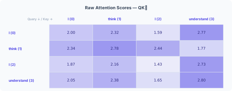
4.3. Step 1 — Compare every Query against every Key
for our four tokens, using the Q and K matrices from module 3:
4.4. Step 2 — Scale and softmax
Divide every entry by , then take the softmax of each row:
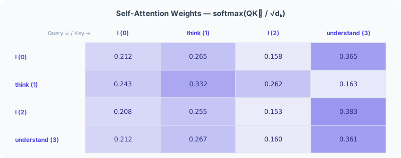
Every row sums to 1.0 — it's a full probability distribution over "how much should I borrow from each token." Notice "think" is the outlier: it attends to itself (33.2%) more than to anything else, while the other three tokens all lean most heavily on "understand."
4.5. Step 3 — Blend the Values
Multiply the weight matrix by to get the final, context-aware output — one blended vector per token:
| Word (pos) | Self-Attention Output |
|---|---|
| I (0) | [0.695, 2.329] |
| think (1) | [0.667, 2.258] |
| I (2) | [0.699, 2.333] |
| understand (3) | [0.695, 2.328] |
The two "I" rows are now extremely close to each other — [0.695, 2.329] versus [0.699, 2.333] — but still not identical. That tiny remaining gap is the last trace of a difference that started all the way back in module 2's positional encoding, carried through Q, K, and V, and survived the blending step. In a real model, later layers (and multiple attention heads, next module) amplify differences like this rather than let them wash out.
def softmax(x, axis=-1):
    x = x - np.max(x, axis=axis, keepdims=True)
    e = np.exp(x)
    return e / np.sum(e, axis=axis, keepdims=True)

d_k = K.shape[-1]
scores = Q @ K.T / np.sqrt(d_k)
weights = softmax(scores, axis=-1)
output = weights @ V

print(np.round(weights, 3))
# [[0.212 0.265 0.158 0.365]
#  [0.243 0.332 0.262 0.163]
#  [0.208 0.255 0.153 0.383]
#  [0.212 0.267 0.16  0.361]]

print(np.round(output, 3))
# [[0.695 2.329]
#  [0.667 2.258]
#  [0.699 2.333]
#  [0.695 2.328]]
4.6. Causal masking (for decoder-style models)
Everything above is bidirectional self-attention — every token can see every other token, including ones that come after it. That's fine for a model that gets to look at the whole sentence at once (an encoder, like BERT [2]). But a model that generates text one token at a time (a decoder, like GPT [3]) can't be allowed to peek at future tokens during training — at generation time, those tokens don't exist yet. The fix is a causal mask: before the softmax, block every (query, key) pair where the key comes after the query.
The usual way to write it is to add a mask matrix to the scaled scores before the softmax, where is 0 for allowed positions and for blocked ones:
Adding to a score forces its softmax output to exactly 0 — the position is completely blocked, not just discouraged. Row of only leaves columns through open, so token can only attend to itself and whatever came before it:
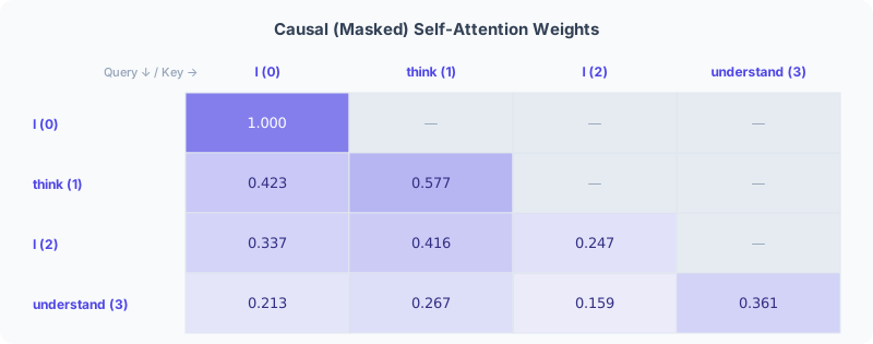
Compare "think" (position 1) in both versions. Unmasked, it split its attention across all four tokens: [0.243, 0.332, 0.262, 0.163]. Masked, it can only see "I" (0) and itself: [0.423, 0.577, 0, 0] — and its output changes from [0.667, 2.258] to [0.648, 2.304] as a result. "understand" (3), on the other hand, is completely unaffected by the mask — it's the last token, so nothing was ever in its future to block.
seq_len = Q.shape[0]
future = np.triu(np.ones((seq_len, seq_len), dtype=bool), k=1)
masked_scores = np.where(future, -np.inf, scores)

masked_weights = softmax(masked_scores, axis=-1)
masked_output = masked_weights @ V

print(np.round(masked_weights, 3))
# [[1.    0.    0.    0.   ]
#  [0.423 0.577 0.    0.   ]
#  [0.337 0.416 0.247 0.   ]
#  [0.213 0.267 0.159 0.361]]

print(np.round(masked_output, 3))
# [[1.    1.75 ]
#  [0.648 2.304]
#  [0.66  2.206]
#  [0.695 2.329]]
Note:
np.triu(..., k=1)marks the strictly-upper-triangular positions — the "future" ones. Usingnp.whereto set those to (rather than multiplying a 0/1 mask by ) sidesteps a classic bug: isNaNin IEEE floating point, not0.
4.7. Up next: multi-head attention
Each token now has a single output vector that blends in information from the rest of the sentence (or, with masking, from itself and everything before it). But every token used the same Q/K/V projections to do this — one fixed "way of looking." The next module, multi-head attention, runs several of these attention computations in parallel, each with its own projections, so the model can track several different kinds of relationships at once — then a feed-forward layer processes each token's result individually before the next Transformer block begins.
5. Multi-Head Attention
5.1. Why multiple heads
Module 4 ran attention exactly once, with one fixed , , . That forces every token to judge "relevance" the same single way for every kind of relationship in the sentence — but real language has several kinds of relationships at once (what refers to what, what modifies what, what's simply nearby). One shared projection has to compromise across all of them.
Multi-head attention runs several attention computations in parallel, on the same input, each with its own learned , , — so each head is free to specialize. Their outputs are then concatenated and mixed back together with one more learned projection.
5.2. The multi-head formula
With heads and model dimension , each head usually projects down to , so that concatenating all heads of size adds back up to exactly — ready for the next Transformer block. In our example, and , so — which is exactly the single-head setup modules 3 and 4 already built. That computation is head 1. We just need a head 2, and a way to combine them.
5.3. Head 2 — a different point of view
Head 2 gets its own weight matrices — same shapes as head 1's, but mixing the input dimensions differently:
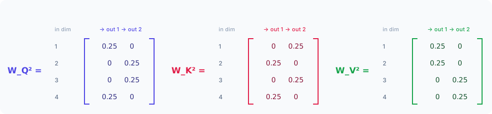
Projecting the same position-aware embedding matrix through these gives head 2's own Q, K, and V:
| Word (pos) | Query (Q²) | Key (K²) | Value (V²) |
|---|---|---|---|
| I (0) | [1.00, 1.00] | [1.00, 1.00] | [0.50, 1.50] |
| think (1) | [1.96, 0.39] | [1.14, 1.21] | [1.59, 0.75] |
| I (2) | [1.23, 0.65] | [0.65, 1.23] | [0.37, 1.50] |
| understand (3) | [1.29, 0.76] | [1.75, 0.29] | [0.54, 1.51] |
Same recipe as module 4 — , scale by , softmax each row:
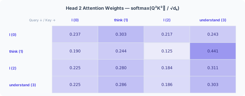
Multiplying those weights by gives head 2's output — a second, independent blended vector per token:
| Word (pos) | Head 2 Output |
|---|---|
| I (0) | [0.812, 1.275] |
| think (1) | [0.768, 1.321] |
| I (2) | [0.793, 1.293] |
| understand (3) | [0.800, 1.288] |
Compare "think" across the two heads: head 1 attended to itself most (33.2%); head 2 attends to "understand" most (44.1%). Same token, same sentence, same formula — two different heads noticed two different things.
5.4. Concatenate and project
Stick each token's two head outputs together into one 4-dimensional vector:
| Word (pos) | head 1 | head 2 | Concatenated |
|---|---|---|---|
| I (0) | [0.695, 2.329] | [0.812, 1.275] | [0.695, 2.329, 0.812, 1.275] |
| think (1) | [0.667, 2.258] | [0.768, 1.321] | [0.667, 2.258, 0.768, 1.321] |
| I (2) | [0.699, 2.333] | [0.793, 1.293] | [0.699, 2.333, 0.793, 1.293] |
| understand (3) | [0.695, 2.328] | [0.800, 1.288] | [0.695, 2.328, 0.800, 1.288] |
Then multiply by the output projection — the piece from Equation (11) that lets the model actually combine what the two heads found, rather than just stacking them side by side untouched:
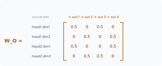
Worked example for "I" at position 0:
The same projection, applied to all four tokens, gives the final output of the multi-head attention layer:
| Word (pos) | Multi-Head Attention Output |
|---|---|
| I (0) | [0.754, 1.802, 0.985, 1.571] |
| think (1) | [0.718, 1.789, 0.994, 1.513] |
| I (2) | [0.746, 1.813, 0.996, 1.563] |
| understand (3) | [0.748, 1.808, 0.992, 1.564] |
Back to — the same shape the block started with. That's what makes Transformer blocks stackable: this output is a legal input to another identical block.
Note: restoring is specifically 's job, not the feed-forward layer's — and it isn't a free choice. Every Transformer block wraps its sub-layers in a residual connection, , and that addition only works if the two shapes match exactly. So must map the concatenated heads () back to — which is also why was never a free choice either, back in Equation (10). By the time the feed-forward layer (next) receives its input, it's already -shaped; the FFN's own internal widen-then-narrow pattern (, typically ) is a separate design choice for extra per-token capacity, not a fix-up for anything multi-head attention left undone.
def self_attention(Q, K, V):
    d_k = K.shape[-1]
    scores = Q @ K.T / np.sqrt(d_k)
    weights = softmax(scores, axis=-1)
    return weights @ V

def multi_head_attention(X, heads, W_O):
    # heads: list of (W_Q, W_K, W_V) for each head
    outputs = []
    for W_Q, W_K, W_V in heads:
        Q, K, V = X @ W_Q, X @ W_K, X @ W_V
        outputs.append(self_attention(Q, K, V))
    concat = np.concatenate(outputs, axis=-1)
    return concat @ W_O

heads = [
    (W_Q, W_K, W_V),      # head 1 — from module 3
    (W_Q2, W_K2, W_V2),   # head 2
]

output = multi_head_attention(position_aware_embeddings, heads, W_O)
print(np.round(output, 3))
# [[0.754 1.802 0.985 1.571]
#  [0.718 1.789 0.994 1.513]
#  [0.746 1.813 0.996 1.563]
#  [0.748 1.808 0.992 1.564]]
5.5. Up next: the feed-forward layer
Each token now carries a representation shaped by two different heads' worth of "what matters to me." The next piece of a Transformer block, a position-wise feed-forward network, processes each token's vector individually (no cross-token mixing this time) — and then, wrapped together with residual connections and normalization, this becomes one complete encoder block. From there, the last remaining piece is the decoder: what changes when a model has to generate rather than just read — masked self-attention (built already, back in module 4) plus a new sub-layer, cross-attention, where Queries come from the decoder and Keys/Values come from the encoder's output.
6. Feed-Forward Network
6.1. Why a feed-forward layer
Self-attention and multi-head attention are the only places information moves between tokens — every other step so far (embedding lookup, adding positional encoding, projecting Q/K/V) works on one token at a time. The feed-forward network is the same kind of per-token step: it takes each token's multi-head attention output and transforms it individually, with no knowledge of what any other token's vector looks like. Attention decides what to gather from the sentence; the feed-forward layer gives each token extra capacity to process what it gathered.
It's a small two-layer network applied identically to every token: a linear projection up to a wider hidden dimension, a non-linearity, then a linear projection back down:
is ReLU — the original "Attention Is All You Need" paper's choice (modern models often swap in GELU [4] or a gated variant, but the shape of the computation is the same). has shape and has shape , so the vector widens on the way in and narrows back down on the way out. Real models typically use (mentioned already in the note back in module 5). We use here — 1.5x rather than 4x — purely so the weight matrices stay small enough to read at a glance; the arithmetic is identical either way.
6.2. Example weights
, . projects up:
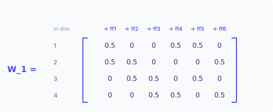
projects back down:
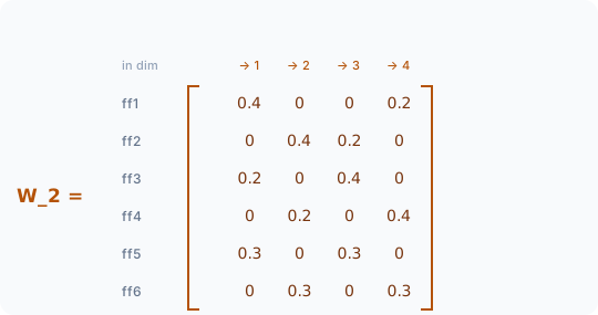
The negative biases in are deliberate — they're picked so that ReLU actually clips something in the next step, instead of every value quietly staying positive and the non-linearity doing nothing visible.
6.3. Step 1 — Widen: project up to and apply ReLU
Starting from module 5's multi-head attention output, run each token through Equation (12)'s first half, :
| Word (pos) | Pre-activation () |
|---|---|
| I (0) | [0.278, 0.194, 0.278, -0.137, -0.031, 0.587] |
| think (1) | [0.253, 0.192, 0.253, -0.185, -0.044, 0.551] |
| I (2) | [0.280, 0.205, 0.280, -0.145, -0.029, 0.588] |
| understand (3) | [0.278, 0.200, 0.278, -0.144, -0.030, 0.586] |
ReLU zeroes out every negative entry and leaves the rest untouched. For all four tokens, dimensions ff4 and ff5 are negative and get clipped to 0 — that's expected given how close these four multi-head attention outputs already are to each other (module 5 flagged this: three of the four rows are nearly identical):
| Word (pos) | After ReLU |
|---|---|
| I (0) | [0.278, 0.194, 0.278, 0.000, 0.000, 0.587] |
| think (1) | [0.253, 0.192, 0.253, 0.000, 0.000, 0.551] |
| I (2) | [0.280, 0.205, 0.280, 0.000, 0.000, 0.588] |
| understand (3) | [0.278, 0.200, 0.278, 0.000, 0.000, 0.586] |
6.4. Step 2 — Narrow: project back down to
Multiplying by and adding — the second half of Equation (12) — brings each token back to a 4-dimensional vector:
| Word (pos) | FFN Output () |
|---|---|
| I (0) | [0.267, 0.353, 0.250, 0.332] |
| think (1) | [0.252, 0.342, 0.240, 0.316] |
| I (2) | [0.268, 0.358, 0.253, 0.332] |
| understand (3) | [0.267, 0.356, 0.251, 0.331] |
Every token went through the exact same , , , — nothing here mixes information across rows. Compare that to self-attention, where every output row was a blend of all four input rows.
import numpy as np

W1 = np.array([
    [0.5, 0,   0,   0.5, 0.5, 0  ],
    [0.5, 0.5, 0,   0,   0,   0.5],
    [0,   0.5, 0.5, 0,   0.5, 0  ],
    [0,   0,   0.5, 0.5, 0,   0.5],
])
b1 = np.array([-1.0, -1.2, -1.0, -1.3, -0.9, -1.1])

W2 = np.array([
    [0.4, 0,   0,   0.2],
    [0,   0.4, 0.2, 0  ],
    [0.2, 0,   0.4, 0  ],
    [0,   0.2, 0,   0.4],
    [0.3, 0,   0.3, 0  ],
    [0,   0.3, 0,   0.3],
])
b2 = np.array([0.1, 0.1, 0.1, 0.1])

def feed_forward(x):
    hidden = np.maximum(0, x @ W1 + b1)
    return hidden @ W2 + b2

ffn_output = feed_forward(output)  # `output` is module 5's multi-head attention result
print(np.round(ffn_output, 3))
# [[0.267 0.353 0.25  0.332]
#  [0.252 0.342 0.24  0.316]
#  [0.268 0.358 0.253 0.332]
#  [0.267 0.356 0.251 0.331]]
6.5. Residual connections and layer normalization
Every sub-layer we've built so far — multi-head attention, and now the feed-forward network — is wrapped the same way in a real Transformer block: add the sub-layer's input back to its output (a residual connection [5]), then normalize:
This is the formula the note back in module 5 referenced without a number. Two things are packed into it:
- Residual connection () — adding the sub-layer's own input back to its output. This is what makes very deep stacks of Transformer blocks trainable: even if a sub-layer's gradient signal is weak, the
+xterm gives the gradient an unobstructed path straight through, so it doesn't vanish over dozens of stacked blocks. - Layer normalization [6] — re-centers and re-scales each token's vector independently, so the numbers flowing into the next sub-layer stay in a stable, consistent range no matter how many blocks deep you are:
is element-wise multiplication — pair up with the normalized vector dimension by dimension and multiply, the same way the that follows pairs up dimension by dimension and adds (unlike the matrix multiplications everywhere else in this post, nothing here mixes across dimensions). and are the mean and variance of a single token's vector, computed across its own dimensions (not across tokens — each row is normalized independently, same "no cross-token mixing" rule as the feed-forward layer). is a tiny constant ( or so) just to avoid dividing by zero. and are learned per-dimension scale and shift — we use , below, which makes Equation (13) a pure normalization with nothing learned added on top.
Worked example for "I" at position 0. is its multi-head attention output (module 5), and is the FFN output we just computed:
| Value | |
|---|---|
[0.754, 1.802, 0.985, 1.571] | |
[0.267, 0.353, 0.250, 0.332] | |
[1.021, 2.155, 1.235, 1.903] | |
| mean , variance | 1.578, 0.217 |
| LayerNorm output | [-1.198, 1.239, -0.738, 0.696] |
The same steps, for all four tokens:
| Word (pos) | LayerNorm Output | |
|---|---|---|
| I (0) | [1.021, 2.155, 1.235, 1.903] | [-1.198, 1.239, -0.738, 0.696] |
| think (1) | [0.970, 2.131, 1.234, 1.829] | [-1.237, 1.279, -0.666, 0.624] |
| I (2) | [1.014, 2.171, 1.249, 1.895] | [-1.213, 1.256, -0.711, 0.668] |
| understand (3) | [1.015, 2.164, 1.243, 1.895] | [-1.208, 1.251, -0.719, 0.677] |
Every row now has mean 0 and unit variance — LayerNorm has no interest in the scale of a token's vector, only its shape relative to itself.
def layer_norm(x, gamma=1.0, beta=0.0, eps=1e-6):
    mu = x.mean(axis=-1, keepdims=True)
    var = x.var(axis=-1, keepdims=True)
    return gamma * (x - mu) / np.sqrt(var + eps) + beta

add_norm_output = layer_norm(output + ffn_output)
print(np.round(add_norm_output, 3))
# [[-1.198  1.239 -0.738  0.696]
#  [-1.237  1.279 -0.666  0.624]
#  [-1.213  1.256 -0.711  0.668]
#  [-1.208  1.251 -0.719  0.677]]
Note: a real encoder block applies this Add & Norm step twice — once after multi-head attention, once after the feed-forward network. To keep modules 4 and 5 focused on attention itself, this post's earlier multi-head attention output was left un-normalized; the formula for that first Add & Norm is identical to Equation (14), just with = the position-aware embeddings and = multi-head attention's output. Figure 14 below assembles both.
6.6. Assembling a full encoder block
Putting every module in this post together, in order, is one complete Transformer encoder block:
- Token embedding (module 1) + positional encoding (module 2) →
- Multi-head self-attention (module 3, 4, 5) on
- Add & Norm:
- Feed-forward network (this module) on the result of step 3
- Add & Norm:
Step 5's output is -shaped, same as — so it's a legal input to another block with the same structure:
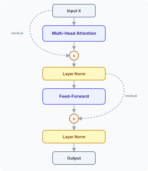
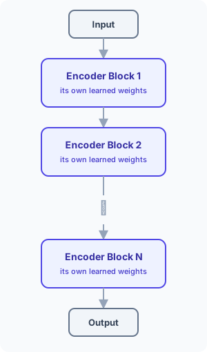
Real models stack several of these (6, 12, 24, ...) one after another — but "stacked" doesn't mean one block runs in a loop, reusing the same weights. Every position in the stack gets its own independently learned , , , , , , , and ; block 5 has no idea what block 2 learned. They're separate blocks that just happen to share the identical five-step shape diagrammed above:
6.7. Up next: the decoder
That's every sub-layer an encoder block needs, worked by hand: embeddings, positional encoding, Q/K/V, self-attention with optional causal masking, multi-head attention, the feed-forward network, and the residual-plus-normalization wrapper tying it all together. The last piece of the series is the decoder — which reuses masked self-attention (already built, back in module 4) and adds one new sub-layer, cross-attention, where Queries come from the decoder while Keys and Values come from this encoder's output. That's how a decoder-based model like a translator gets to look back at the source sentence while generating its output one token at a time.
References
- [1]Vaswani et al. (2017). Attention Is All You Need. Conference on Neural Information Processing Systems (NeurIPS).
- [2]Devlin et al. (2018). BERT: Pre-training of Deep Bidirectional Transformers for Language Understanding. Conference of the North American Chapter of the Association for Computational Linguistics: Human Language Technologies (NAACL-HLT).
- [3]Radford et al. (2018). Improving Language Understanding by Generative Pre-Training. OpenAI.
- [4]Hendrycks & Gimpel (2016). Gaussian Error Linear Units (GELUs).
- [5]He et al. (2015). Deep Residual Learning for Image Recognition. IEEE Conference on Computer Vision and Pattern Recognition (CVPR).
- [6]Ba, Kiros & Hinton (2016). Layer Normalization.