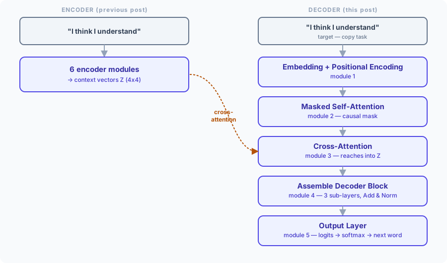
The encoder post worked through six modules that turn a sentence into a stack of context-aware vectors — token embeddings, positional encoding, Q/K/V, self-attention, multi-head attention, and a feed-forward network, wrapped up into a repeatable encoder block. This post picks up right where that one left off and covers the other half of the Transformer: the decoder, the part that actually produces output, one token at a time.
To keep this post connected to the last one instead of introducing an unrelated new example, the decoder's job throughout is the simplest one there is: reproduce the exact sentence the encoder just read. This "copy task" is a classic toy setup for studying attention mechanisms — trivial for a person, but it makes it easy to verify, step by step, that the decoder's attention is actually pointing at the right place, since we already know what the right answer looks like.
Same ground rules as before: a tiny 4-dimensional toy example, worked by hand, with a runnable Python snippet at every step. We'll reuse the same 6-word vocabulary and embedding table from the encoder post's first module, so there's no new setup to learn before the real content starts.
Contents
- Decoder input — embedding and positional encoding for the target sequence (covered below)
- Masked self-attention — the causal-masking mechanism from the encoder post, applied to the decoder's own input (covered below)
- Cross-attention — the decoder's new sub-layer, attending to the encoder's output (covered below)
- Assembling a full decoder block — three sub-layers, three residual-and-norm wrappers (covered below)
- The output layer — projecting back to vocabulary size and generating a sequence (covered below)
1. Decoder Input
1.1. What the decoder actually receives
The encoder's input was fixed from the start: the whole source sentence, all at once. The decoder's input is different — it's the target sequence, the thing the model is producing. During training, that's the correct output shifted right by one position (so the model never sees the token it's about to predict); during actual generation, it's simply whatever the model has produced so far, one token longer on every pass.
That shift-and-generate mechanic matters a lot once we get to actually producing output, so we'll come back to it in the output-layer module. For now, to keep this module focused on the mechanism rather than the bookkeeping, we'll just work with a plain target sequence — no shifting yet — and build it up exactly the same way module 1 of the encoder post built up its input.
1.2. The example sequence
Instead of inventing a new, unrelated sentence, let's give the decoder the simplest possible job: reproduce the exact sentence the encoder just read.
I think I understand
Same 4 tokens, same IDs as the encoder post's own example: [0, 1, 0, 2]. This "copy task" is a deliberately easy target — the payoff comes later, once cross-attention is built, when it becomes trivial to sanity-check whether the mechanism is doing the right thing (decoder position 0, predicting "I", ought to attend strongly back to the encoder's "I" positions — and we'll be able to check that directly).
1.3. Steps 1-3 — Embedding, positional encoding, and adding them together
Since it's the exact same 4-token sequence at the exact same 4 positions, every number here is identical to what the encoder post already computed in its own modules 1 and 2 — embedding lookup and positional encoding are both pure functions of (word, position), so re-running them on the same input can only produce the same output:
| Word (pos) | Decoder Input |
|---|---|
| I (0) | [1.00, 1.00, 3.00, 3.00] |
| think (1) | [4.84, 1.54, 0.01, 3.00] |
| I (2) | [1.91, -0.42, 3.02, 3.00] |
| understand (3) | [0.14, 2.01, 1.03, 5.00] |
If you want the tokenization step, the embedding table, or the positional encoding formula worked out by hand, they're in the encoder post's modules 1 and 2 — Equation (1) and Equation (2) are the exact formulas reused here.
Note: this numerical overlap is a side effect of choosing a copy task, not a general rule. The decoder's embedding and positional encoding are a completely separate computation from the encoder's, run on the decoder's own input — they only happen to land on the same numbers here because the input happens to be the same sentence. In a real translation model the target would be a different sentence, quite possibly in a different language, and none of these numbers would match the encoder's.
import numpy as np

embedding_table = np.array([
    [1, 0, 3, 2],  # I
    [4, 1, 0, 2],  # think
    [0, 3, 1, 4],  # understand
    [2, 2, 4, 0],  # love
    [3, 0, 2, 1],  # dog
    [1, 4, 0, 3],  # cat
])

def positional_encoding(seq_len, d_model):
    positions = np.arange(seq_len)[:, None]
    dims = np.arange(d_model)[None, :]
    angle_rates = 1 / np.power(10000, (2 * (dims // 2)) / d_model)
    angles = positions * angle_rates
    pe = np.zeros((seq_len, d_model))
    pe[:, 0::2] = np.sin(angles[:, 0::2])
    pe[:, 1::2] = np.cos(angles[:, 1::2])
    return pe

target_ids = [0, 1, 0, 2]  # "I", "think", "I", "understand" — the copy-task target
target_embeddings = embedding_table[target_ids]
pe = positional_encoding(seq_len=4, d_model=4)

decoder_input = target_embeddings + pe
print(np.round(decoder_input, 2))
# [[1.   1.   3.   3.  ]
#  [4.84 1.54 0.01 3.  ]
#  [1.91 -0.42 3.02 3.  ]
#  [0.14 2.01 1.03 5.  ]]
1.4. Up next: masked self-attention
The decoder now has its own 4x4 position-aware input matrix — numerically identical to the encoder's, for this example, but conceptually its own computation. The next step runs self-attention across it, with the causal mask from the encoder post's module 4 back in play, since the decoder generates left to right and can never be allowed to peek at a token it hasn't produced yet.
2. Masked Self-Attention
2.1. The same mechanism, the decoder's own weights
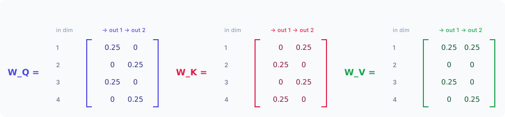
This is exactly the masked self-attention mechanism from the encoder post's module 4 — Equation (8) — applied here to the decoder's own input. The only genuinely new thing is which weights are doing the projecting: the decoder learns its own , , , separate from the encoder's, even though — thanks to the copy task — both sides happen to start from the same input numbers this time.
2.2. Why the mask isn't optional here
The encoder post introduced causal masking as something an encoder could use, depending on the task — encoders that read the whole input at once, like BERT [1], usually skip it. For a decoder, masking isn't a design choice; it's a requirement. The decoder generates its output left to right, one token at a time, and at generation time, token 3 simply doesn't exist yet when the model is producing token 1. Training has to respect that same restriction, or the model would learn to lean on future tokens it will never actually have at inference time. Every decoder, in every Transformer, masks its self-attention for exactly this reason.
2.3. Example weights
, , and below are the decoder's own, 4x2 each — same shape as the encoder's Q/K/V weights, different learned numbers:
2.4. Step 1 — Project into Q, K, V
The same projection as module 3 of the encoder post, applied to the decoder's own input and its own weights:
| Word (pos) | Query (Q) | Key (K) | Value (V) |
|---|---|---|---|
| I (0) | [1.00, 1.00] | [1.00, 1.00] | [1.00, 1.00] |
| think (1) | [1.21, 1.14] | [1.14, 1.21] | [1.21, 1.96] |
| I (2) | [1.23, 0.65] | [0.65, 1.23] | [1.23, 1.23] |
| understand (3) | [0.29, 1.75] | [1.75, 0.29] | [0.29, 1.29] |
2.5. Step 2 — Scale, mask, and softmax
Same recipe as before: , divide by , add the mask matrix — Equation (9), unchanged, since the decoder's target here is also 4 tokens long — then softmax each row:
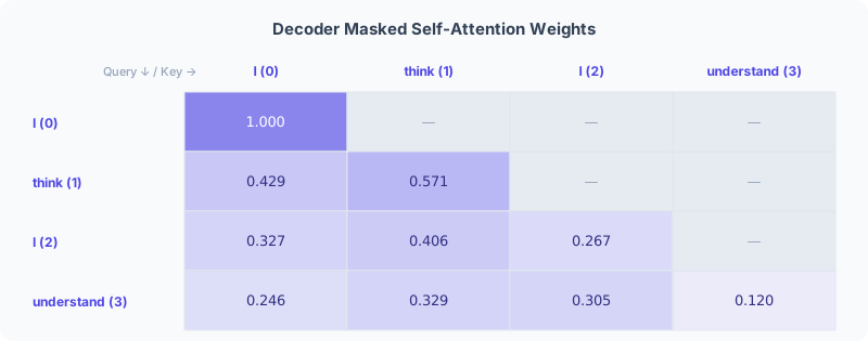
Same lower-triangular shape as the encoder post's masked example, for the same reason: row only leaves columns through open, so each token can only pull from itself and whatever came before it. "I" at position 0 has nowhere else to look, so its weight is trivially 1.000; by position 3, "understand" is blending all four tokens (itself included) with weights [0.246, 0.329, 0.305, 0.120].
2.6. Step 3 — Blend the values
Multiply the masked weights by to get the decoder's own masked self-attention output:
| Word (pos) | Masked Self-Attention Output |
|---|---|
| I (0) | [1.000, 1.000] |
| think (1) | [1.121, 1.548] |
| I (2) | [1.148, 1.450] |
| understand (3) | [1.056, 1.420] |
Note: the 4x4 matrix above is the training view — the whole target sequence fed in at once, with the mask hiding the future from a model that technically already has the answer in front of it, and all four rows coming out of one parallel matrix multiplication (exactly why Transformers train faster than RNNs, which really were forced to go one step at a time). At actual generation time there's no full sequence to feed in yet, so the decoder builds it up one token at a time — 1x4, then 2x4, then 3x4, then 4x4, self-attending fresh at each step. Careful with that "4," though: the second number is , the embedding width, which never changes no matter how long the sequence gets; the first number is the sequence length, and it only happens to also reach 4 here because we picked a 4-token target for the copy task — a coincidence of this toy example, not a consequence of . The model doesn't know in advance to stop at 4 tokens either — it stops when it generates a learned end-of-sequence token, with an external max-length cap as a backstop in case it never does. Module 5 covers that generation loop, stopping condition included.
def softmax(x, axis=-1):
    x = x - np.max(x, axis=axis, keepdims=True)
    e = np.exp(x)
    return e / np.sum(e, axis=axis, keepdims=True)

W_Q = np.array([[0.25, 0], [0, 0.25], [0.25, 0], [0, 0.25]])
W_K = np.array([[0, 0.25], [0.25, 0], [0, 0.25], [0.25, 0]])
W_V = np.array([[0.25, 0.25], [0, 0], [0.25, 0], [0, 0.25]])

Q = decoder_input @ W_Q
K = decoder_input @ W_K
V = decoder_input @ W_V

d_k = K.shape[-1]
scores = Q @ K.T / np.sqrt(d_k)

seq_len = Q.shape[0]
future = np.triu(np.ones((seq_len, seq_len), dtype=bool), k=1)
masked_scores = np.where(future, -np.inf, scores)

weights = softmax(masked_scores, axis=-1)
masked_output = weights @ V

print(np.round(weights, 3))
# [[1.    0.    0.    0.   ]
#  [0.429 0.571 0.    0.   ]
#  [0.327 0.406 0.267 0.   ]
#  [0.246 0.329 0.305 0.12 ]]

print(np.round(masked_output, 3))
# [[1.    1.   ]
#  [1.121 1.548]
#  [1.148 1.45 ]
#  [1.056 1.42 ]]
2.7. Up next: cross-attention
Every token in the decoder now carries a representation built purely from other decoder tokens — the same sentence, self-attending to itself, causally masked. But that's not enough to be useful: right now the decoder has no way to actually look at the source sentence it's supposed to be working from. That's the one genuinely new sub-layer in a decoder block, and it's next: cross-attention, where Queries come from the decoder and Keys and Values come from the encoder's output — the from the very first module of the encoder post, finally coming back into play.
3. Cross-Attention
3.1. The one genuinely new sub-layer
Masked self-attention let decoder tokens look at each other — but only at each other. The decoder still has no way to actually use the sentence it's supposed to be working from. That's cross-attention's whole job: Queries come from the decoder, but Keys and Values come from the encoder's finished output, .
The attention formula itself doesn't change at all — it's still exactly Equation (7), . The only thing that's different is where the three inputs come from:
That's the entire mechanism, really. Self-attention, masked or not, always projects Q, K, and V from the same sequence. Equation (1) deliberately splits that apart: Q comes from one sequence (the decoder), K and V come from a completely different one (the encoder). Everything downstream — the dot products, the scaling, the softmax, the blending — is the formula you already know.
3.2. Why K and V share a source, but Q doesn't
K and V always have to come from the same place; Q doesn't, and that's not an arbitrary rule. Attention scores relevance using K, then retrieves content using V — position in K and position in V only make sense together if they describe the same item. A library's index card and book #47 have to actually be the same library's book #47, or scoring one and fetching from the other wouldn't correspond to anything. Q has no such constraint, since it isn't paired positionally with anything — it's compared against every K position at once, not matched one-to-one — so it's free to come from an entirely different sequence.
Seen this way, self-attention isn't really a separate mechanism from cross-attention; it's just the special case where all three happen to come from the same place. Cross-attention is what happens when K and V stay paired together while Q comes from somewhere else.
3.3. Why the decoder is the one asking
That "somewhere else" is specifically the decoder — not, say, the encoder borrowing a query out of the decoder's side instead. That direction is fixed too, and for a good reason.
At any point during generation, Q is built from whatever the decoder has produced so far: the query genuinely comes from the output side, already-generated words asking a question, not from the source sentence. That can feel backwards at first — shouldn't the source, the thing being translated from, be the one doing the searching?
But attention direction follows whoever currently has a state that's changing. The encoder's output is finished the moment the encoder runs, and never changes again for the rest of decoding. The decoder's situation is the opposite: it's different at every step, because a little more of the translation exists each time. Only the side with a changing "where am I right now" state can meaningfully ask a question — the fixed side can only sit there and answer.
Picture translating "I think I understand" into French, partway through, having already produced "Je pense" (I think). To generate the next word, the decoder needs to ask something like given that I've covered "I think" already, what part of the source is still unaddressed? Only the decoder's own current state knows that "Je pense" is what's done so far — the source sentence has no notion of "which part has been translated"; it's just sitting there, complete, waiting to be consulted.
It's not only semantics, either — it's a computational necessity. The encoder runs once, up front, before decoding even starts, and produces one fixed that gets reused identically at every decoding step: token 1's cross-attention reaches into , token 2's reaches into that same , and so on. If the direction were reversed — supplying the query, the decoder supplying K and V — would need to query into a decoder state that doesn't exist yet at the moment it's computed, since decoding hasn't even started. "Encode once, decode incrementally" only works if the thing computed once is the fixed lookup table (K and V) and the thing that changes at every step is what does the asking (Q).
3.4. No mask this time
Module 2's masking existed because the decoder's own sequence is being generated left to right — token 3 doesn't exist yet when the model is producing token 1. None of that applies to the source sentence. The encoder read the whole thing before generation even started; there's no "future" token in to hide, because was never generated incrementally in the first place. Every decoder position is free to attend to every encoder position, always — cross-attention is never masked.
3.5. Where Q, K, and V actually come from here
and are projected from , the encoder's finished output — the result of "Assembling a full encoder block" back in the encoder post.
is projected from the decoder's own representation. In a complete decoder block, that would be the output of masked self-attention, after its own multi-head wrapping and Add & Norm — module 4 assembles that full chain. To keep this module focused on the one new thing, cross-attention itself, we'll project directly from the decoder's original input (module 1's result) instead — dimensionally identical, and the mechanism doesn't care which upstream computation handed it a 4-dimensional vector.
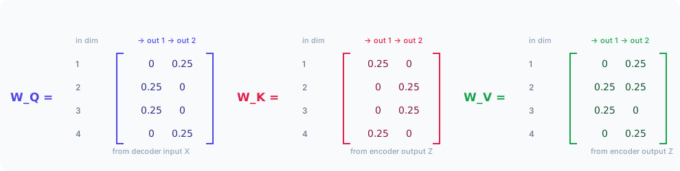
3.6. Cross-attention's own weights
3.7. Step 1 — Project Q from the decoder, K and V from the encoder
| Word (pos) | Query (Q), from decoder | Key (K), from encoder | Value (V), from encoder |
|---|---|---|---|
| I (0) | [1.00, 1.00] | [-0.13, 0.13] | [0.13, 0.18] |
| think (1) | [0.39, 1.96] | [-0.15, 0.15] | [0.15, 0.17] |
| I (2) | [0.65, 1.23] | [-0.14, 0.14] | [0.14, 0.18] |
| understand (3) | [0.76, 1.29] | [-0.13, 0.13] | [0.13, 0.18] |
Notice the four Key rows (and Value rows) are all nearly identical to each other. That's not a computation error — it's a direct consequence of itself: by the end of the encoder post, all four of its output tokens had converged to be extremely close to each other (a side effect of this toy example's small, hand-picked weights, flagged back when that table was first computed). Feed cross-attention four nearly-identical keys, and there's very little left for it to tell apart.
3.8. Step 2 — Scale and softmax (no mask to apply)
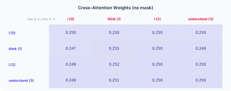
Exactly as predicted: the weights are almost perfectly uniform, every row hovering right around across all four columns. This is cross-attention doing its job correctly, not failing — it's only as selective as the differences between the keys it's given, and here those differences are tiny. In a real trained model, the encoder's output tokens stay meaningfully distinct from each other (that differentiation is part of what training the encoder actually teaches it to do), so cross-attention in practice produces exactly the kind of sharp, interpretable "look here" pattern this small hand-picked example can't quite show.
3.9. Step 3 — Blend the encoder's values
| Word (pos) | Cross-Attention Output |
|---|---|
| I (0) | [0.1369, 0.1771] |
| think (1) | [0.1371, 0.1771] |
| I (2) | [0.1370, 0.1771] |
| understand (3) | [0.1370, 0.1771] |
Four outputs that are, again, nearly identical — the direct downstream consequence of nearly-uniform attention over nearly-identical values. Every decoder position ends up pulling back roughly the same blend of the encoder's output, because there wasn't much of a real difference to pull apart in the first place.
Z = np.array([
    [-1.198, 1.239, -0.738, 0.696],
    [-1.237, 1.279, -0.666, 0.624],
    [-1.213, 1.256, -0.711, 0.668],
    [-1.208, 1.251, -0.719, 0.677],
])  # the encoder post's final output

W_Q = np.array([[0, 0.25], [0.25, 0], [0.25, 0], [0, 0.25]])
W_K = np.array([[0.25, 0], [0, 0.25], [0, 0.25], [0.25, 0]])
W_V = np.array([[0, 0.25], [0.25, 0.25], [0.25, 0], [0, 0.25]])

Q = decoder_input @ W_Q
K = Z @ W_K
V = Z @ W_V

d_k = K.shape[-1]
scores = Q @ K.T / np.sqrt(d_k)
weights = softmax(scores, axis=-1)  # no mask
cross_output = weights @ V

print(np.round(weights, 4))
# [[0.25   0.25   0.25   0.25  ]
#  [0.2467 0.2546 0.2498 0.2489]
#  [0.2488 0.2517 0.2499 0.2496]
#  [0.2489 0.2515 0.2499 0.2497]]

print(np.round(cross_output, 4))
# [[0.1369 0.1771]
#  [0.1371 0.1771]
#  [0.137  0.1771]
#  [0.137  0.1771]]
3.10. Up next: assembling a full decoder block
Every sub-layer a decoder block needs now exists: masked self-attention, cross-attention, and the feed-forward network (already built, back in the encoder post — it's identical regardless of which side of the model it runs on). What's left is wiring them together in order, each one wrapped in its own residual connection and layer norm, the same way the encoder post's module 6 assembled its own block.
4. Assembling a Full Decoder Block
4.1. Three sub-layers instead of two
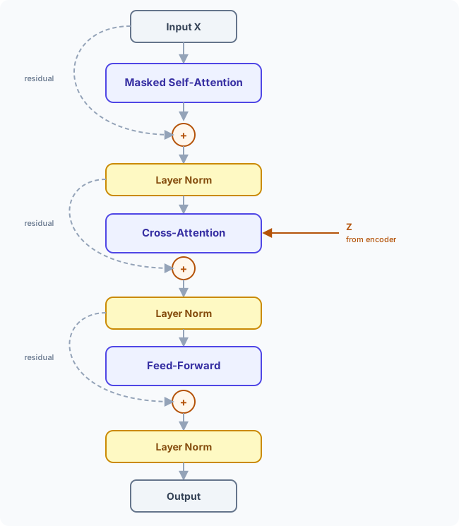
A decoder block wraps three sub-layers in residual connections and layer norms, not two — masked self-attention, cross-attention, and the feed-forward network, each followed by its own Add & Norm. Everything needed for all three already exists: masked self-attention from module 2, cross-attention from module 3, and the feed-forward network with its residual-plus-normalization wrapper, Equation (14), both reused directly from the encoder post.
4.2. Restoring before the residual add
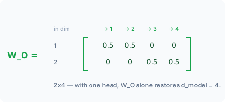
Modules 2 and 3 both used a single attention head, landing at — the same simplification the encoder post's own module 4 made before module 5 introduced multiple heads. Add & Norm needs the sub-layer's output to match 's shape, , so the two can be added element-wise. In a full model that's 's job (real decoders typically run several heads through both attention sub-layers too, exactly like the encoder post's module 5 — nothing new to re-derive, since concatenating heads and projecting with is the identical mechanism no matter how many heads feed into it). With a single head, "concatenating" is trivial — there's only one thing to concatenate — so alone does the work, projecting straight from up to .
4.3. Worked example: Add & Norm after masked self-attention
Projecting module 2's output through , adding it back to , then normalizing:
| Word (pos) | Sublayer(X), via | + Sublayer(X) | LayerNorm Output |
|---|---|---|---|
| I (0) | [0.500, 0.500, 0.500, 0.500] | [1.500, 1.500, 3.500, 3.500] | [-1.000, -1.000, 1.000, 1.000] |
| think (1) | [0.560, 0.560, 0.774, 0.774] | [5.401, 2.101, 0.784, 3.774] | [1.373, -0.526, -1.284, 0.437] |
| I (2) | [0.574, 0.574, 0.725, 0.725] | [2.484, 0.154, 3.745, 3.725] | [-0.029, -1.623, 0.833, 0.819] |
| understand (3) | [0.528, 0.528, 0.710, 0.710] | [0.668, 2.538, 1.740, 5.710] | [-1.062, -0.067, -0.492, 1.621] |
This is Equation (14), unchanged — . Only what counts as is new here.
W_O_masked = np.array([[0.5, 0.5, 0, 0], [0, 0, 0.5, 0.5]])

sublayer_out = masked_output @ W_O_masked  # masked_output from module 2
residual = decoder_input + sublayer_out    # decoder_input from module 1

def layer_norm(x, gamma=1.0, beta=0.0, eps=1e-6):
    mu = x.mean(axis=-1, keepdims=True)
    var = x.var(axis=-1, keepdims=True)
    return gamma * (x - mu) / np.sqrt(var + eps) + beta

add_norm_1 = layer_norm(residual)
print(np.round(add_norm_1, 3))
# [[-1.    -1.     1.     1.   ]
#  [ 1.373 -0.526 -1.284  0.437]
#  [-0.029 -1.623  0.833  0.819]
#  [-1.062 -0.067 -0.492  1.621]]
4.4. The same wrap, twice more
Cross-attention gets identical treatment: its own, separately learned restores , then . The feed-forward network — reused directly from the encoder post's module 6, since it's identical regardless of which side of the model it runs on — gets the same wrap a third time. Neither is recomputed numerically here; the mechanism is exactly the worked example above, just with different weights and a different sub-layer plugged in.
4.5. Assembling the full block
Putting every module in this post together, in order, is one complete Transformer decoder block:
- Decoder input (module 1) →
- Masked self-attention (module 2) on
- Add & Norm:
- Cross-attention (module 3) on step 3's output, reaching into the encoder's
- Add & Norm:
- Feed-forward network (from the encoder post) on step 5's output
- Add & Norm:
Note: module 3's own worked example projected cross-attention's Query from directly, as a simplification — step 4 above shows the fully chained version, sourcing it from step 3's output instead. The mechanism and weights are identical either way; only which numbers go in changes. We kept module 3's original numbers rather than redo them here, since that module's job was showing how cross-attention works, not tracing the exact production chain.
Step 7's output is -shaped, same as — ready to feed into another stacked decoder block, or into the last piece of the model: the output layer.
4.6. Up next: the output layer
Every sub-layer a decoder block needs now exists and fits together. What's left is the very last step: turning that final -shaped vector at each position into an actual predicted word — a linear projection back up to vocabulary size, a softmax, and, finally, the shift-and-generate mechanic promised all the way back in module 1.
5. The Output Layer
5.1. From a vector back to a word
Every module so far has kept each token as a -shaped vector — 4 numbers, picking up more context at every step. But 4 numbers aren't a word. The very last piece of the model is a linear layer that projects that vector up to the size of the vocabulary, giving one raw score — a logit — per word, then a softmax turns those scores into an actual probability distribution to pick a word from:
Equation (2) is just one more linear projection, the same shape of operation as every , , , or / already used in this series — the only thing that changes is the output width, which is no longer or , but the entire vocabulary.
5.2. 's shape
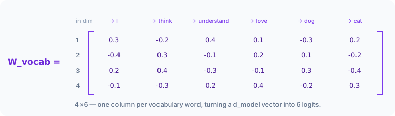
has shape — 4x6 here, since our toy vocabulary only has 6 words. Real models project up to tens or hundreds of thousands of columns, one per subword token (and often reuse the embedding table itself, transposed, as — a trick called weight tying [2] that saves a full set of parameters, since both matrices are already shaped to map between the same two spaces).
5.3. Worked example: from decoder representation to word probabilities
Module 4 assembled the full three-sub-layer chain conceptually but didn't recompute it numerically end to end. Rather than invent a new cross-attention and re-derive fresh numbers just to demonstrate this one, final, independent step, we reuse module 4's own worked Add & Norm output — the table from "Worked example: Add & Norm after masked self-attention" — as the stand-in decoder representation feeding the output layer. Same simplification module 3 already made for cross-attention's Query, for the same reason: this module's job is showing how the projection works, not re-tracing the exact production chain.
Worked out for "I" at position 0:
| Step | Value |
|---|---|
[-1.000, -1.000, 1.000, 1.000] | |
[0.200, 0.000, -0.400, 0.000, 0.300, -0.100] | |
| = logits | [0.300, 0.100, -0.200, -0.100, 0.100, -0.200] |
[0.221, 0.181, 0.134, 0.148, 0.181, 0.134] |
The same steps, for all four positions — each row is a full probability distribution over the 6-word vocabulary, in the order (I, think, understand, love, dog, cat):
| Word (pos) | Logits | |
|---|---|---|
| I (0) | [0.300, 0.100, -0.200, -0.100, 0.100, -0.200] | [0.221, 0.181, 0.134, 0.148, 0.181, 0.134] |
| think (1) | [0.422, -0.977, 1.274, 0.235, -1.137, 0.925] | [0.159, 0.039, 0.373, 0.132, 0.034, 0.263] |
| I (2) | [0.825, -0.294, 0.265, -0.183, -0.268, 0.131] | [0.323, 0.106, 0.184, 0.118, 0.108, 0.161] |
| understand (3) | [-0.452, -0.391, 0.254, 0.478, -0.360, 0.384] | [0.100, 0.106, 0.202, 0.253, 0.109, 0.230] |
Taking the highest-probability word at each position gives "I", "understand", "I", "love" — which doesn't match the copy task's actual target ("think", "I", "understand", the-next-thing) at all. That's expected, not a bug: here is hand-picked, not trained, same as every other weight matrix in this series. A trained model's would have learned, through millions of examples, which decoder representations should map to which words; ours has learned nothing, so its guesses are close to arbitrary. What this worked example demonstrates is purely the mechanism — any -shaped vector deterministically becomes a full probability distribution over the vocabulary through one linear projection and one softmax.
add_norm_1 = np.array([
    [-1.000, -1.000, 1.000, 1.000],
    [1.373, -0.526, -1.284, 0.437],
    [-0.029, -1.623, 0.833, 0.819],
    [-1.062, -0.067, -0.492, 1.621],
])  # module 4's Add & Norm output, reused here

vocab = ["I", "think", "understand", "love", "dog", "cat"]

W_vocab = np.array([
    [0.3, -0.2, 0.4, 0.1, -0.3, 0.2],
    [-0.4, 0.3, -0.1, 0.2, 0.1, -0.2],
    [0.2, 0.4, -0.3, -0.1, 0.3, -0.4],
    [-0.1, -0.3, 0.2, 0.4, -0.2, 0.3],
])
b_vocab = np.array([0.1, 0.1, 0.2, -0.1, -0.2, -0.1])

logits = add_norm_1 @ W_vocab + b_vocab
probs = softmax(logits, axis=-1)
predictions = [vocab[i] for i in np.argmax(probs, axis=-1)]

print(np.round(probs, 3))
# [[0.221 0.181 0.134 0.148 0.181 0.134]
#  [0.159 0.039 0.373 0.132 0.034 0.263]
#  [0.323 0.106 0.184 0.118 0.108 0.161]
#  [0.1   0.106 0.202 0.253 0.109 0.23 ]]

print(predictions)
# ['I', 'understand', 'I', 'love']
5.4. Picking a word: greedy decoding
Taking the single highest-probability word, as the worked example above just did, is called greedy decoding — simple, deterministic, and the easiest way to turn a probability distribution into an actual choice. Real generation systems often do something fancier: sampling from the distribution instead of always taking the top pick (optionally reshaped by a "temperature" that makes the distribution sharper or flatter), or beam search [3], which tracks several candidate sequences at once instead of committing to one word at a time. Those are all strategies for the same underlying question — which word do we commit to, given this distribution — not changes to anything covered so far. Greedy decoding is enough to see the mechanism clearly.
5.5. Training input: teacher forcing and the shift
Module 1 deferred one detail: the decoder's input during training isn't the plain target sequence we've been using throughout this post — it's the target shifted right by one position, with a special beginning-of-sequence token, <BOS>, prepended and the last target token dropped. Position 's input becomes target token , and the model's job at every position is to predict target token — the word that would come next. Feed the model "<BOS> I think I" and it should predict "I", "think", "I", "understand" at positions 0 through 3, respectively, each conditioned only on the shifted input up to that point.
This is why masked self-attention isn't optional (module 2's point again, now with the full picture): with the shifted input and the causal mask together, one single parallel pass over the whole sequence computes correct training predictions for every position at once, each one legitimately blind to the position it's trying to predict. That parallelism, across every position and every training example, is the whole reason Transformers train dramatically faster than the one-token-at-a-time recurrent models that came before them.
5.6. Inference: generating one token at a time
At generation time there's no target to shift — the whole point is that the model doesn't know the answer yet. Generation starts from just <BOS>, runs the entire decoder stack — embedding, positional encoding, masked self-attention, cross-attention into the encoder's , the feed-forward network, and this output layer — on that single-token input, and reads off the probability distribution at the one position that exists. Whatever word gets picked is appended to the input, and the whole stack runs again on the now two-token sequence, reading off the distribution at the new last position. Each pass feeds the entire sequence-so-far back through from scratch (real systems cache the previously computed Keys and Values instead of redoing that work every step — a speed optimization called KV-caching [4], not a change to the mechanism itself).
For our copy task, here's what that loop looks like — illustrating what a genuinely trained model would produce at each step, not the untrained toy from the worked example above:
| Step | Decoder input so far | Predicted next word |
|---|---|---|
| 1 | <BOS> | I |
| 2 | <BOS> I | think |
| 3 | <BOS> I think | I |
| 4 | <BOS> I think I | understand |
| 5 | <BOS> I think I understand | <EOS> |
Each row's input is exactly one token longer than the last, and each pass only ever needs the probability distribution at the final position — everything before it was already decided on a previous step.
5.7. Knowing when to stop
Module 2 flagged this and deferred it here: <EOS> (end-of-sequence) isn't a special mechanism bolted on top — it's just one more entry in the vocabulary, sitting in the same softmax output as "I" or "understand," with its own column in . A trained model learns to assign <EOS> high probability once it judges the sequence complete, and generation simply stops the moment <EOS> is the word that gets picked, same as any other step in the loop above.
That answers the earlier question about knowing the maximum length in advance: nothing is fixed ahead of time. The "4" that showed up repeatedly earlier in this post — the training-time sequence length — was only ever a property of this particular toy sentence, not something the model calculates or commits to beforehand. At actual generation time the sequence grows for as long as the model keeps declining to predict <EOS>. The only fixed number is a backstop max-length cap, applied by the surrounding system rather than the model itself, purely to guarantee termination if <EOS> never comes — an out-of-distribution input, a model that hasn't fully converged, or simply an unlucky generation.
5.8. From sentence to sentence
That completes the whole pipeline diagrammed back in Figure 1: the encoder post's six modules turn "I think I understand" into context vectors ; this post's five modules turn that same sentence, plus , into a decoder block whose output layer predicts, one word at a time, the very sentence the encoder started with. The copy task made that connection checkable at every step along the way — masked self-attention only pulling from earlier positions, cross-attention reaching back into , and finally, here, a probability distribution that would, in a trained model, hand back "I think I understand" one predicted word at a time. Every mechanism between those two sentences is now the same mechanism running inside GPT [5], Whisper [6], and Claude [7].
References
- [1]Devlin et al. (2018). BERT: Pre-training of Deep Bidirectional Transformers for Language Understanding. Conference of the North American Chapter of the Association for Computational Linguistics: Human Language Technologies (NAACL-HLT).
- [2]Press & Wolf (2017). Using the Output Embedding to Improve Language Models. Conference of the European Chapter of the Association for Computational Linguistics (EACL).
- [3]Sutskever, Vinyals & Le (2014). Sequence to Sequence Learning with Neural Networks. Conference on Neural Information Processing Systems (NeurIPS).
- [4]Pope et al. (2022). Efficiently Scaling Transformer Inference. Conference on Machine Learning and Systems (MLSys).
- [5]Radford et al. (2018). Improving Language Understanding by Generative Pre-Training. OpenAI.
- [6]Radford et al. (2022). Robust Speech Recognition via Large-Scale Weak Supervision. International Conference on Machine Learning (ICML).
- [7]Anthropic (2024). Claude.