Classical 3D reconstruction — structure from motion, multi-view stereo, TSDF fusion — stores a scene explicitly: a point cloud, a mesh, a voxel grid. Every one of those representations makes the same trade: resolution is fixed by how many points, triangles, or voxels you're willing to allocate, and anything the sensor never saw stays a hole. NeRF [1] throws that trade out entirely. A scene isn't stored anywhere as geometry at all — it's the weights of a small neural network, queryable at any continuous 3D point, that answers "how much stuff is here, and what color does it emit toward the camera." Nothing is discretized until the very last step, when that continuous field gets rendered into a 2D image.

This post works through exactly how that rendering step works — the volume rendering integral, and the discrete approximation of it that actually runs on a GPU — since that's the one piece of machinery a background in explicit reconstruction doesn't hand you for free. It's also the piece worth understanding on its own terms before looking at Gaussian Splatting [4], which keeps NeRF's "render by compositing along a ray" idea but throws out the neural field and the per-pixel network queries that make NeRF slow — a contrast that only lands once it's clear what NeRF is actually paying for.

From Explicit Geometry to an Implicit Radiance Field — what a coordinate network stores, and how it differs from a point cloud, mesh, or voxel grid
Casting Rays Through the Field — the ray equation, density as absorption, and transmittance as a survival probability
The Volume Rendering Integral — the equation that turns a ray's density and color into a pixel, and where it actually comes from
From Integral to Quadrature: A Worked Example — the discrete formula real implementations use, worked by hand on a four-sample toy ray
Positional Encoding: Giving the MLP High Frequencies — why raw coordinates blur, and the sin/cos trick that fixes it
Hierarchical Volume Sampling — spending network evaluations where the ray actually has something to render
The Network and the View-Dependence Split — why density never sees viewing direction, and color always does
Training: A Fully Differentiable Renderer — the loss, and why every step above has to be differentiable
What NeRF Costs, and Why That Matters — the per-pixel price of an implicit field, and what an explicit alternative would trade away

1. From Explicit Geometry to an Implicit Radiance Field

1.1. What "explicit" reconstruction stores

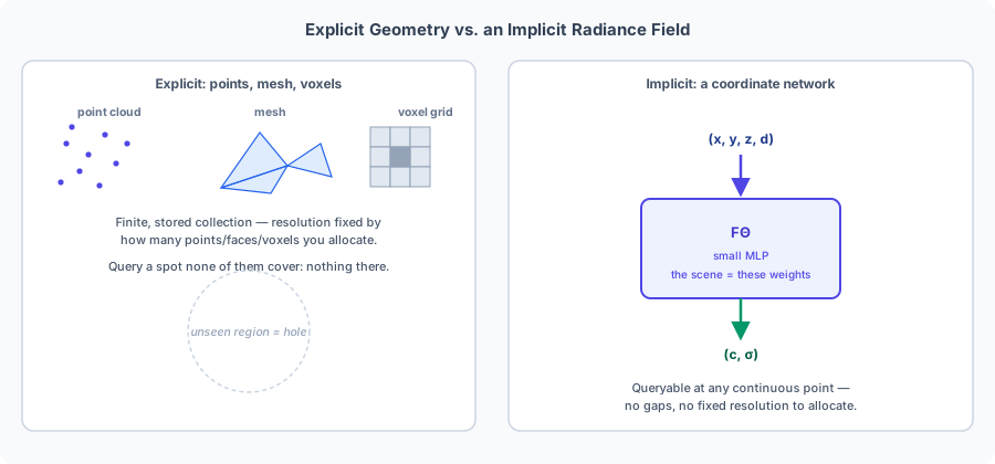
A point cloud from structure-from-motion, a mesh from Poisson reconstruction, a TSDF (Truncated Signed Distance Function — a voxel grid where each cell stores a distance to the nearest surface, positive in front of it and negative behind, truncated to a narrow band around the surface so only nearby cells carry a meaningful value) volume from KinectFusion-style depth fusion — all of these store geometry as a finite, explicit collection of things: 3D points, triangles, or voxel cells, each carrying its own attributes. Query a location the collection doesn't cover — a spot no camera saw, a gap between voxels — and there's simply nothing there. More detail means allocating more points, more triangles, or a finer voxel grid; resolution and memory are the same knob.

Diagram contrasting explicit 3D representations with an implicit neural field — Figure 1. Explicit representations — point clouds, meshes, voxel grids, TSDFs — store geometry directly, at a resolution fixed by how many points or voxels you allocate. A neural radiance field stores nothing explicit at all: the scene is the weights of a small MLP, queryable at any continuous 3D point.

1.2. A scene as a function, not a collection

NeRF replaces the collection with a function. A coordinate network — a plain multilayer perceptron, no convolutions, no explicit spatial structure — takes a 3D point and a viewing direction and returns a color and a density:

F_{Θ} : (x, d) \mapsto (c, σ) (1)

$x = (x, y, z)$ is a 3D position, $d$ a viewing direction (a unit vector), $c$ the emitted RGB color, and $σ$ the volume density — how opaque space is at that point. Its units are inverse length, and that's not an arbitrary convention: multiplied by a small travel distance $d t$ , $σ d t$ gives a dimensionless probability of the ray being absorbed over that stretch (Section 2.2 makes this precise). So $σ$ itself reads as a rate of absorption per unit distance — near zero through empty space, where a ray can travel indefinitely without being stopped, and large inside solid material, where a ray is absorbed within a very short distance. $Θ$ is just the network's weights. There's no point cloud, no mesh, no voxel grid anywhere in this picture: the scene is $Θ$ , and "querying the reconstruction" means one forward pass through a small MLP. Resolution isn't a stored quantity at all — $F_{Θ}$ can be evaluated at any $(x, d)$ , including ones nothing in the training data landed on exactly, the same way an SDF (Signed Distance Function — the same idea as the TSDF above, minus the truncation) can be evaluated at any point even though it was fit from a finite set of depth samples.

That continuity is the whole appeal, and it comes with a cost this post spends real time on: producing a 2D image from $F_{Θ}$ means integrating it along a ray, and that integral has no closed form for an arbitrary network. Sections 2 through 4 build up exactly what has to be computed, and how it's actually approximated.

2. Casting Rays Through the Field

2.1. The ray equation

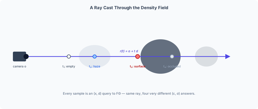
A camera ray through one pixel is exactly what it is in any multi-view geometry pipeline — an origin $o$ (the camera center) and a unit direction $d$ (from the pixel's back-projected ray), swept out by a scalar $t$ :

r (t) = o + t d, t_{n} \leq t \leq t_{f} (2)

$t_{n}$ and $t_{f}$ are near and far bounds — nothing needs to be rendered outside them. Nothing here is new if rays and camera centers are already familiar; the new part starts with what happens along the ray.

A camera ray passing through a volume of density, with sample points marked along it — Figure 2. A ray r(t) = o + td cast from the camera through one pixel, passing through the density field. Sample points along the ray are where the network gets queried for (c, σ) — empty space, a partially transparent region, and a solid surface all along the same ray.

2.2. Density as absorption, and transmittance as survival

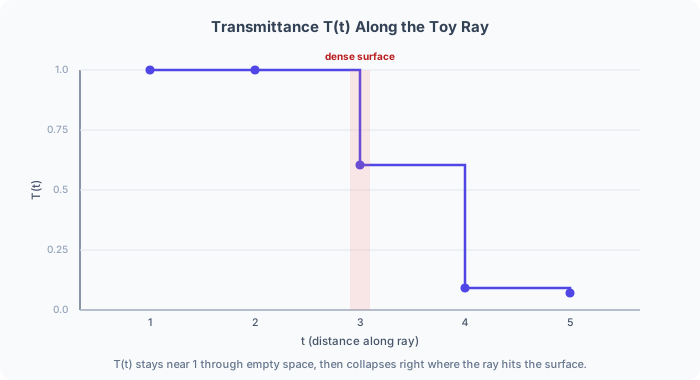
Treat $σ (x)$ as a literal absorption coefficient, the same quantity that appears in the Beer-Lambert law governing light passing through fog, smoke, or tissue in a CT scan: the probability of the ray being absorbed in an infinitesimal segment $d t$ at position $r (t)$ is $σ (r (t)) d t$ . Beer-Lambert says the fraction of light surviving a segment decays exponentially with accumulated density, which gives transmittance — the probability the ray travels all the way from $t_{n}$ to $t$ without being absorbed:

T (t) = exp (- \int_{t_{n}}^{t} σ (r (s)) d s) (3)

$T (t_{n}) = 1$ — nothing has been absorbed yet, right at the camera. As $t$ increases through empty space ( $σ \approx 0$ ), $T (t)$ barely moves. The moment the ray crosses genuinely solid material ( $σ$ large), the integral inside the exponential grows fast and $T (t)$ collapses toward zero — exactly the statement "once the ray has hit something opaque, nothing behind it can still influence the pixel."

Plot of transmittance T(t) decaying to zero as a ray passes through a dense surface — Figure 3. Transmittance T(t) starts at 1 (nothing absorbed yet) and decays as accumulated density builds up along the ray. It drops sharply where the ray crosses a solid surface, and levels off near zero behind it — samples back there can no longer affect the rendered color.

3. The Volume Rendering Integral

3.1. Combining survival, termination, and color

A ray contributes color to a pixel at exactly the point it terminates — gets absorbed or scattered back toward the camera. The probability of that happening in the infinitesimal window $[t, t + d t]$ is the probability of surviving up to $t$ , times the probability of terminating in that next sliver: $T (t) σ (r (t)) d t$ . Weight the color emitted there, $c (r (t), d)$ , by that probability, and integrate over every point the ray could terminate at, and the result is the pixel's expected color:

C (r) = \int_{t_{n}}^{t_{f}} T (t) σ (r (t)) c (r (t), d) d t (4)

Diagram breaking the volume rendering integral's three factors apart — Figure 4. The volume rendering integral's integrand as three multiplied factors: T(t), the probability of surviving to t; σ(r(t))dt, the probability of terminating in the next dt; and c(r(t), d), the color emitted there. Their product, integrated over the ray, is the pixel color.

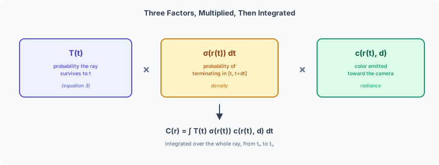
Nothing about Equation (4) is new to NeRF — it's the classical emission-absorption optical model used for direct volume rendering in medical visualization and graphics for decades before neural networks entered the picture [2]. NeRF's actual contribution is narrower and more specific: let $σ$ and $c$ be the outputs of a neural network (Equation (1)) instead of a hand-specified transfer function over a voxel grid, and make the whole rendering pipeline differentiable end to end, so that a rendering error — a rendered pixel compared against a real photograph — can be backpropagated all the way into $Θ$ . That's the training story in Section 8; first, Equation (4) itself has no closed form for a network as $F_{Θ}$ , so it has to be approximated numerically before it's usable at all.

4. From Integral to Quadrature: A Worked Example

4.1. Stratified sampling and the discrete formula

Equation (4) can't be integrated symbolically — $σ$ and $c$ are whatever an MLP happens to output, not a function with a known antiderivative. The fix is numerical quadrature: partition $[t_{n}, t_{f}]$ into $N$ bins and draw one sample per bin (stratified sampling — one random sample inside each bin, rather than one fixed sample per bin, so that across training iterations the network effectively gets queried at a continuum of positions, not a fixed discrete grid). Query $F_{Θ}$ at each sample $t_{i}$ to get $σ_{i}$ and $c_{i}$ , then approximate the integral as:

δ_{i} = t_{i + 1} - t_{i}, α_{i} = 1 - exp (- σ_{i} δ_{i}), T_{i} = j = 1 \prod i - 1 (1 - α_{j}), \hat{C} (r) = i = 1 \sum N T_{i} α_{i} c_{i} (5)

$α_{i}$ is the local opacity of sample $i$ — how much of the ray's remaining light gets absorbed in just that one interval — and $T_{i}$ is the discrete transmittance, the fraction of light that survived every interval before this one. This is exactly the standard graphics alpha compositing ("over") operator, applied back-to-front along the ray: composite $N$ semi-transparent layers, each with its own color and opacity, and $T_{i} α_{i}$ is precisely the weight layer $i$ ends up contributing to the final blended pixel.

Note: $σ_{i}$ isn't itself a probability — it's unbounded above, the way a density can be, not a value in $[0, 1]$ ; $α_{i}$ is what's actually bounded there, and it takes both $σ_{i}$ and $δ_{i}$ to get it. The exponential also saturates smoothly as $σ_{i}$ grows, so $α_{i} \to 1$ without ever overshooting — the bound that's actually enforced is the other end, $σ \geq 0$ via a ReLU/softplus on the network's output, since a negative $σ$ would push $α_{i}$ negative too.

4.2. A four-sample toy ray, by hand

Take a ray with four samples, evenly spaced at $t = 1, 2, 3, 4$ with a far bound at $t = 5$ (so every $δ_{i} = 1$ , keeping the arithmetic on one line). Pick densities and colors — collapsed to a single scalar intensity rather than full RGB, since the compositing math is identical per-channel — that tell a simple story: mostly empty space, then a dense surface, then something behind it that the surface should occlude:

$i$	$t_{i}$	$σ_{i}$	$c_{i}$	reading
1	1	0.0	0.2	empty space
2	2	0.5	0.4	thin haze
3	3	2.0	0.9	a dense, bright surface
4	4	0.1	0.1	dark, and behind the surface

import numpy as np

t = np.array([1.0, 2.0, 3.0, 4.0])
sigma = np.array([0.0, 0.5, 2.0, 0.1])
c = np.array([0.2, 0.4, 0.9, 0.1])
delta = np.array([1.0, 1.0, 1.0, 1.0])   # t=5 far bound makes every interval width 1

alpha = 1.0 - np.exp(-sigma * delta)
# shift right by one, prepend T_1 = 1, drop the last (unused) transmittance
T = np.concatenate([[1.0], np.cumprod(1.0 - alpha)[:-1]])
weights = T * alpha

C_hat = np.sum(weights * c)

print("alpha  ", np.round(alpha, 3))
print("T      ", np.round(T, 3))
print("weights", np.round(weights, 3))
print("sum(w) ", round(float(weights.sum()), 3))
print("C_hat  ", round(float(C_hat), 3))
# alpha   [0.    0.393 0.865 0.095]
# T       [1.    1.    0.607 0.082]
# weights [0.    0.393 0.524 0.008]
# sum(w)  0.926
# C_hat   0.63

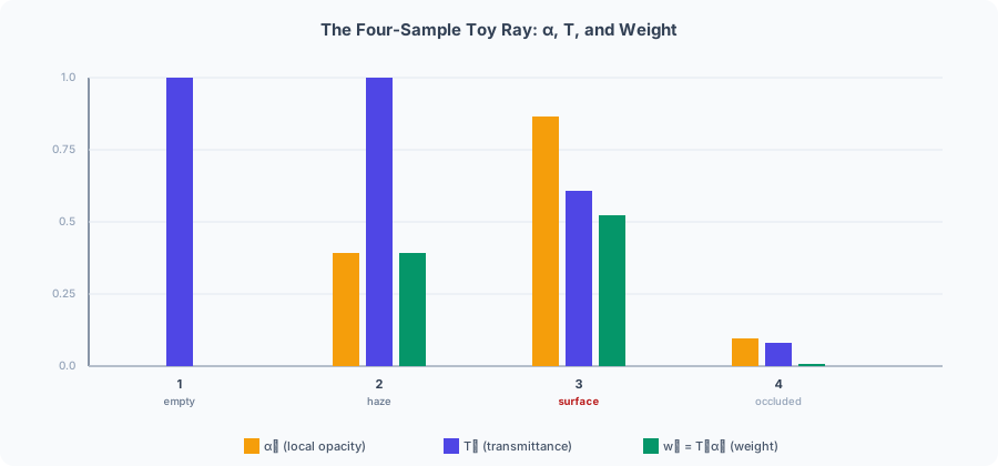
Bar chart of density, alpha, transmittance, and weight for the four-sample toy ray — Figure 5. The toy ray's four samples: raw density σ_i, local opacity α_i, accumulated transmittance T_i, and final compositing weight w_i = T_iα_i. Sample 3, the dense surface, dominates the weight; sample 4, sitting behind it, contributes almost nothing.

Read the weights column: sample 1 contributes nothing ( $α_{1} = 0$ — empty space absorbs nothing). Sample 2's haze contributes a modest 0.393. Sample 3, the dense surface, dominates at 0.524 — most of the final color comes from here. Sample 4 sits right behind the surface and barely registers, 0.008, because $T_{4} = 0.082$ : by the time the ray reaches it, 92% of the ray's "light" has already been absorbed by sample 3. That's occlusion, falling directly out of Equation (5) with no separate visibility test required — a dense sample earlier on the ray automatically suppresses whatever comes after it, just by shrinking $T$ for every later $i$ , continuously — not a hard cutoff: a semi-transparent sample only partially dims what's behind it, in proportion to its own $α$ .

The weights don't sum to exactly 1 — they sum to 0.926, because $T_{5} \approx 0.074$ of the ray's "light" survives past $t = 4$ without being absorbed anywhere. In a real renderer that remainder either composites over a background color or is left as-is, depending on the scene; it's the same quantity the accumulated-opacity channel of a compositing pipeline tracks.

5. Positional Encoding: Giving the MLP High Frequencies

5.1. Why raw coordinates blur

Feeding $(x, y, z)$ directly into an MLP produces reconstructions that are systematically oversmoothed — sharp edges and fine texture come out blurry no matter how long training runs. MLPs have a well-documented bias toward learning low-frequency functions first and struggle to represent high-frequency variation from low-dimensional inputs like a raw 3D coordinate [3]. A single scalar $x$ changes smoothly and slowly as it varies — there's no way for a few dot products and ReLUs downstream of it to suddenly produce a sharp edge at some specific $x$ without an enormous number of units doing exactly that.

5.2. Mapping a coordinate through sinusoids

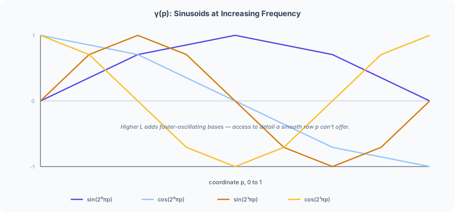
The fix doesn't touch the network at all — it maps each input coordinate through a fixed bank of sinusoids at exponentially increasing frequencies before the MLP ever sees it:

γ (p) = (sin (2^{0} π p), cos (2^{0} π p), \dots, sin (2^{L - 1} π p), cos (2^{L - 1} π p)) (6)

applied independently to each of $x$ , $y$ , $z$ (NeRF uses $L = 10$ , so each 3D position becomes a $3 \times 2 \times 10 = 60$ -dimensional vector) and, separately, to each of the three components of the unit viewing direction $d$ ( $L = 4$ , so $3 \times 2 \times 4 = 24$ dimensions). A worked example with $L = 2$ on a single coordinate $p = 0.3$ :

import numpy as np

p, L = 0.3, 2
freqs = 2.0 ** np.arange(L)          # [1, 2]
angles = np.pi * p * freqs           # [0.9425, 1.8850] radians
gamma = np.stack([np.sin(angles), np.cos(angles)], axis=1).flatten()
print(np.round(gamma, 3))
# [ 0.809  0.588  0.951 -0.309]

$γ (0.3) = [0.809, 0.588, 0.951, - 0.309]$ — four numbers out of one, at two different frequencies. Raising $L$ adds higher frequencies still, each one a function that genuinely oscillates fast as $p$ moves — exactly the kind of rapid variation a raw coordinate can't offer the network directly, and exactly what lets the same MLP now represent a sharp edge without needing a disproportionate number of extra units to do it.

Sine and cosine basis functions at increasing frequencies used for positional encoding — Figure 6. The sin/cos basis functions γ(p) evaluates a coordinate against, at exponentially increasing frequencies 2^0, 2^1, …. A raw coordinate is one smooth, low-frequency value; stacking it against these bases gives the MLP direct access to high-frequency detail.

$σ$ in Equation (1) is a function of $γ (x)$ only — never $γ (d)$ . Section 7 comes back to exactly why that split matters.

6. Hierarchical Volume Sampling

6.1. Most of a ray is wasted

The stratified samples from Section 4 are spread uniformly along the whole ray — but most of any given ray passes through either empty space or material already occluded by something closer to the camera. Evaluating the (comparatively expensive) MLP at every one of those uniform samples spends most of the compute budget on positions that end up contributing almost nothing to Equation (5), exactly like sample 4 in Section 4.2's toy ray.

6.2. Coarse weights become a sampling distribution

NeRF runs two networks: a coarse network evaluated at $N_{c}$ uniform stratified samples first, whose weights $w_{i} = T_{i} α_{i}$ (Equation (5)) get treated as a piecewise-constant probability distribution along the ray, describing where the ray is likely to actually matter. $N_{f}$ additional samples are then drawn from that distribution via inverse-CDF sampling, biased toward exactly the high-weight regions the coarse pass already found. The coarse and fine sample sets are combined, and a second, fine network is evaluated on the union to produce the final rendered color.

Note: "coarse" and "fine" aren't different-sized networks — both are the same architecture from Section 7, just two separately-trained sets of weights, $Θ_{c}$ and $Θ_{f}$ . What differs is only which samples each is evaluated on, and its job: the coarse network exists to produce a good importance-sampling distribution, not a good final image.

Reuse Section 4.2's own weights, $w = [0.000, 0.393, 0.524, 0.008]$ , summing to $0.926$ . Normalizing into a distribution and taking the cumulative sum gives the sampling CDF:

weights = np.array([0.0, 0.393, 0.524, 0.008])
pdf = weights / weights.sum()
cdf = np.cumsum(pdf)
print("pdf", np.round(pdf, 3))
print("cdf", np.round(cdf, 3))
# pdf [0.    0.425 0.566 0.009]
# cdf [0.    0.425 0.991 1.   ]

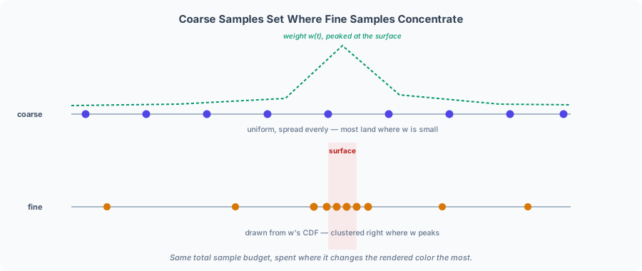
Diagram comparing uniform coarse samples to fine samples concentrated near a surface — Figure 7. Coarse-pass samples spread uniformly along the ray (top) produce a weight distribution that's sharply peaked at the surface. Fine-pass samples (bottom) are then drawn from that distribution, concentrating additional network evaluations exactly where they change the rendered color the most.

The CDF climbs almost all the way to 1 by bin 3 — so a uniform random draw $ξ \sim U (0, 1)$ , inverted through this CDF, lands in bin 2 or bin 3 (the haze and the surface) the overwhelming majority of the time, and essentially never in bin 4, behind the surface. That's the whole point of hierarchical sampling: the fine network's extra evaluations land almost entirely on the region that Section 4.2 already showed dominates the final color, instead of being spread uniformly across a ray that's mostly empty or occluded.

7. The Network and the View-Dependence Split

7.1. Architecture

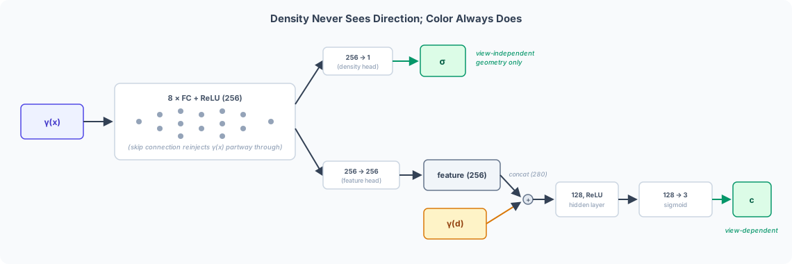
$F_{Θ}$ is a plain MLP, split into two stages. $γ (x)$ (60-dimensional) runs through eight fully-connected layers (256 units each, each one followed by its own ReLU — a nonlinearity has to sit between every pair of linear layers, or the stack collapses into one linear map regardless of how many layers it's written as), with a skip connection reinjecting $γ (x)$ partway through. That shared 256-dimensional trunk output then branches into two separate linear heads, not one: a $256 \to 1$ layer producing $σ$ , and a $256 \to 256$ layer producing a feature vector — two different linear projections of the same trunk output, not the trunk's raw output read twice. Only then does viewing direction enter: that feature vector is concatenated with $γ (d)$ (24-dimensional), giving a 280-dimensional input to one more small hidden layer (128 units, again with its own ReLU), which is in turn projected down to exactly 3 channels by one final linear layer and squashed through a sigmoid to keep each channel in $[0, 1]$ — that last sigmoid output is the RGB color.

Diagram of NeRF's MLP, splitting into a view-independent density head and a view-dependent color head — Figure 8. The positionally-encoded point γ(x) runs through eight ReLU layers to a shared trunk, which branches into two separate linear heads — 256→1 for density σ, 256→256 for a feature vector — neither of which has ever seen the viewing direction. Only the last head mixes that feature with the encoded viewing direction γ(d), through a 128-unit hidden layer and a final 128→3 sigmoid projection, to produce a view-dependent RGB.

7.2. Why density is view-independent and color isn't

$σ$ comes out of the network before $γ (d)$ is ever concatenated in — it's architecturally incapable of depending on viewing direction. That's a deliberate constraint, and it's the neural-field version of an assumption multi-view stereo already leans on: a real surface occupies the same physical location regardless of which camera is looking at it, so geometry predicted from one viewpoint has to agree with geometry predicted from another. Baking that into the architecture — rather than hoping the network learns it — is what makes the recovered "surface" (wherever $σ$ is large) consistent across all the training views.

Color gets the opposite treatment on purpose. Classical multi-view stereo's photo-consistency check generally assumes a Lambertian surface — the same color seen from any direction — and that assumption breaks down on anything glossy or specular, a familiar failure mode from traditional reconstruction pipelines. NeRF lets $c$ depend on $d$ specifically so it can represent specular highlights and other view-dependent appearance, at the cost of deliberately giving up strict photo-consistency for color alone — never for geometry.

8. Training: A Fully Differentiable Renderer

8.1. The loss

Training uses nothing but posed 2D photographs — the same camera poses a structure-from-motion pipeline like COLMAP would already produce — and a simple photometric loss: render a pixel, compare it against the ground-truth photograph at that pixel, for a batch of rays sampled across the training images. Both the coarse and fine renders are supervised, even though only the fine render is used at test time — the coarse network still has to be accurate, since its weights are what Section 6 draws the fine samples from:

L = r \in R \sum [∥ \hat{C}_{c} (r) - C (r) ∥_{2}^{2} + ∥ \hat{C}_{f} (r) - C (r) ∥_{2}^{2}] (7)

No 3D supervision — no depth maps, no point clouds, no ground-truth $σ$ — appears anywhere in Equation (7). Every bit of 3D structure the network ends up with is inferred purely from 2D pixel colors matching across many viewpoints, the same underlying signal multi-view stereo extracts explicitly through feature matching and triangulation.

8.2. Why differentiability is the whole point

Classical ray tracing finds the first surface a ray hits and stops — a hard, discrete decision, not differentiable in any parameter that would let a rendering error flow backward. Every step of Equation (5) is deliberately a smooth arithmetic expression instead: $α_{i} = 1 - exp (- σ_{i} δ_{i})$ is a smooth, differentiable function of $σ_{i}$ , and $\hat{C}$ is a weighted sum, not an if-else over which sample is "the" surface. That's what makes backpropagation through the entire renderer possible — from a rendered pixel, through Equation (5), through $F_{Θ}$ 's forward pass, all the way into $Θ$ itself — and it's the actual mechanism by which nothing more than posed photographs ever produces a 3D-consistent field.

9. What NeRF Costs, and Why That Matters

9.1. The price of an implicit field

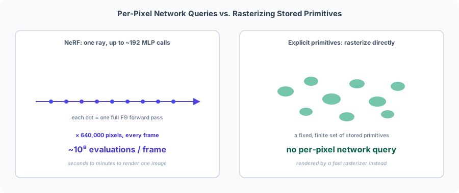
Rendering one pixel means evaluating $F_{Θ}$ at every sample along its ray — $N_{c} + N_{f}$ times, typically 64 coarse plus 128 fine, so up to roughly 192 full MLP forward passes for one pixel. An $800 \times 800$ image is 640,000 pixels; at 192 network evaluations each, a single frame is on the order of $1 0^{8}$ MLP forward passes. Nothing about that cost is a bug to be optimized away later — it's the direct, structural consequence of Section 1's premise: there's no stored geometry to look up, only a function to query, over and over, along every ray, for every frame.

Figure 9. Rendering one NeRF pixel means up to ~192 MLP forward passes along its ray, repeated for every pixel, every frame. An explicit primitive representation, rasterized directly, trades the network queries for a fixed, finite set of stored primitives — the trade the next post takes up directly.

9.2. The alternative

That per-pixel network cost is exactly the bill Gaussian Splatting [4] refuses to pay, by walking Section 1's trade back the other direction: instead of a continuous implicit field queried on demand, store an explicit, finite set of primitives — a return, in spirit, to the point-cloud-shaped representations classical reconstruction already produces — and render them with a fast rasterizer instead of per-pixel ray marching through a network. What stays the same is Equation (5)'s core idea, compositing weighted contributions along a line of sight; what changes is where those contributions come from, and that's the actual subject of the next post.

References

[1]Mildenhall et al. (2020). NeRF: Representing Scenes as Neural Radiance Fields for View Synthesis. European Conference on Computer Vision (ECCV).
[2]Max, N. (1995). Optical Models for Direct Volume Rendering. IEEE Transactions on Visualization and Computer Graphics.
[3]Tancik et al. (2020). Fourier Features Let Networks Learn High Frequency Functions in Low Dimensional Domains. Conference on Neural Information Processing Systems (NeurIPS).
[4]Kerbl et al. (2023). 3D Gaussian Splatting for Real-Time Radiance Field Rendering. ACM Transactions on Graphics (SIGGRAPH).

NeRF: Representing Scenes as Neural Radiance Fields