The Transformer encoder post opened with a specific complaint: RNNs process a sequence one token at a time, so training on a long sequence can't be parallelized across positions. Self-attention fixed that — every position looks at every other position in one matrix multiply, no waiting for a hidden state to arrive from the previous step. But that fix has its own bill, and it comes due at exactly the moment self-attention's parallelism paid off: comparing every position against every other position costs $O (L^{2})$ in the sequence length $L$ , and generating text one token at a time means caching every previous position's key and value vectors forever, a cache that only grows. Mamba [1] is built around a blunt question: what would it take to get a recurrence — one hidden state, updated one token at a time, cost that scales with $L$ and not $L^{2}$ — to actually work as well as attention?

Plain recurrences already existed, and they don't work as well as attention, for a reason this post spends real time on: a fixed-parameter recurrence has no way to look at what token just arrived and decide whether it matters. Mamba's core idea — the "selective" in "selective state space" — is to let the recurrence's own update rule depend on the current input, token by token.

That fix isn't free. Older state-space models trained fast because a fixed recurrence can be rewritten as one convolution and computed over an entire sequence at once — but that rewrite only works if the update rule is the same at every step. Making the rule depend on the input breaks it, which threatens to undo the whole point of moving away from RNNs in the first place. Mamba's second idea, a hardware-aware parallel scan, is what gets that parallel training speed back without giving up selectivity. This post covers both ideas — selection, and the scan that keeps it fast — plus the block that wraps them into something you can actually stack into a language model.

Three-panel comparison of RNN, Transformer, and state space model: training parallelism, per-step inference cost, and memory behavior — Figure 1. An RNN trains sequentially but infers with constant memory. A Transformer trains fully in parallel but its inference cache grows without bound. A state space model is the attempt to get both: a recurrence restructured so it can be trained in parallel too.

This post assumes you've read the Transformer encoder post (self-attention, and why its cost is quadratic) and the decoder post (causal masking and the growing key/value cache at generation time) — both get referenced directly below as the thing Mamba is an alternative to. Nothing here depends on the vision-language posts; Mamba, in its original form, is a language-sequence architecture, not a multimodal one.

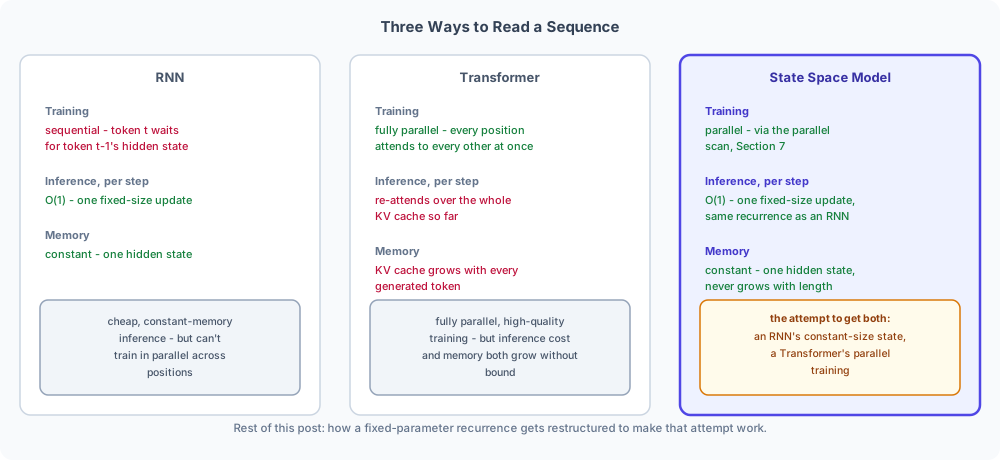
Pick Two: Parallelism, Speed, or Memory — why RNNs, Transformers, and state space models each make a different trade, and what that trade costs as sequences get longer
A State Space Model, One Token at a Time — the continuous equations, a leaky-bucket metaphor for what they mean, and turning a continuous rate into a discrete step
Two Views of the Same Computation — the same recurrence, unrolled into a convolution, and why that convolution is what made pre-Mamba state space models fast to train
Why Fixed Parameters Can't Selectively Remember — the same four tokens, run through a recurrence that can't tell a filler word from a content word
The Selection Mechanism: Let the Input Set the Dials — Δ, B, and C stop being constants and start being functions of the current token
The Price of Selection: No More Convolution — why making the recurrence input-dependent breaks the exact trick that made it fast in the first place
Parallel Scan: Getting Parallelism Back — an associative operator that lets four sequential steps collapse into two parallel rounds
The Mamba Block: Assembling the Layer — expand, branch, gate, project — the whole thing that replaces a Transformer block
What Mamba Buys You, and What It Costs — constant-size inference memory against a growing KV cache, and the one thing attention still does better
Putting It All Together — a minimal reference implementation: discretize, scan, and the full block, in plain NumPy

1. Pick Two: Parallelism, Speed, or Memory

1.1. Three ways to read a sequence

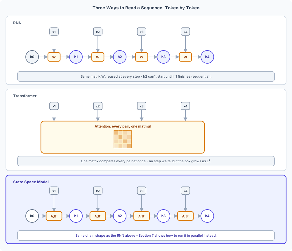
Three families of sequence model exist, and it's worth being blunt about what each one is actually good and bad at before touching a single equation. An RNN keeps a fixed-size hidden state and updates it one token at a time — inference is cheap and memory is constant, but training is sequential, since token 5's hidden state can't be computed before token 4's is. A Transformer looks at every pair of positions at once — training is fully parallel, since every position's output is one matrix multiply away from every other position — but inference means re-attending to a key/value cache that has one entry per previous token, forever growing. A state space model is the attempt to get an RNN's constant-size inference state and a Transformer's parallel training at the same time, by choosing a recurrence simple enough (linear, not the nonlinear gates an LSTM or GRU use) that it can be restructured into a form a GPU can parallelize.

Three rows showing four tokens flowing through an RNN, a Transformer, and a state space model: the RNN and SSM both chain tokens through a small reused matrix one step at a time, while the Transformer feeds all four tokens into one large all-pairs attention matrix at once — Figure 2. The same four tokens, run through each mechanism. An RNN chains them through one small matrix W, reused every step, so h2 has to wait for h1. A Transformer feeds all four into one large matrix at once, no step waiting on another. A state space model chains tokens exactly like the RNN — it's the same shape, just with Ā and B̄ in W's place.

1.2. How cost actually grows with length

The trade in Three ways to read a sequence isn't abstract — it shows up directly in how training compute scales with sequence length $L$ . Self-attention computes an $L \times L$ matrix of pairwise scores, so its cost is $O (L^{2})$ : double the sequence length, and attention gets roughly four times more expensive. A recurrence — RNN or state space model alike — updates a fixed-size state once per token, so its cost is $O (L)$ : double the sequence length, and the cost roughly doubles too, not quadruples.

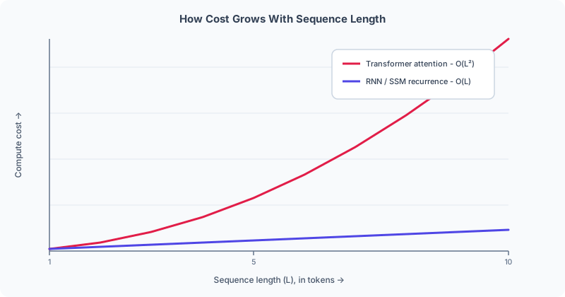
Line plot of compute cost against sequence length, showing a quadratic curve for Transformer self-attention and a straight line for recurrent and state space models — Figure 3. Self-attention compares every position against every other position, so its cost grows quadratically with sequence length. A recurrence updates a fixed-size state once per token, so its cost grows linearly instead.

Nothing about this curve is specific to Mamba — it's the same curve that makes long-context Transformers expensive and is exactly the gap Mamba's recurrence is built to reopen. The rest of this post is about how to build a recurrence that's actually competitive with attention's quality, not just its asymptotics.

2. A State Space Model, One Token at a Time

2.1. The continuous equations, and a bucket to picture them with

A state space model's entire memory is one vector $h (t)$ , updated continuously through a linear differential equation, then read out through a separate linear map:

h^{'} (t) y (t) = A h (t) + B x (t) = C h (t) + D x (t) (1)

$A$ , $B$ , $C$ , $D$ are all just matrices (or a scalar, in $D$ 's case) — no attention, no softmax, nothing nonlinear anywhere in this system. The easiest way to hold onto what it means: picture $h (t)$ as the water level in a bucket. $B x (t)$ is water pouring in, at a rate set by the current input $x (t)$ . $A$ is a leak in the bottom of the bucket — a negative $A$ means water drains out over time, so the bucket "forgets" what it held a while ago unless it keeps getting topped up. $C$ is a dipstick: it doesn't change the water level, it just reads a number off of it, and $D$ is a direct pipe from the input straight to the reading, bypassing the bucket entirely.

Notice that $D$ never touches $h (t)$ — it's a completely separate, direct $x (t) \to y (t)$ shortcut, independent of the bucket, the leak, and everything else in this post that actually does interesting work (discretization, selection, the scan). To keep every worked example focused on the part that matters, this post sets $D = 0$ everywhere from here on — every $y_{t}$ below is computed as plainly $C h_{t}$ , with the $D x_{t}$ term written out once, explicitly, in the very next worked example, so it's visible exactly where it drops out rather than silently missing. Since $D$ never interacts with $h_{t}$ , adding a nonzero $D$ back into any equation or code sample below is always just one independent, final + D * x_t, tacked on after everything else is computed.

2.2. Discretization: turning a rate into a step

Equation (1) describes water level changing every instant, but token sequences are discrete — there is no " $t = 1.5$ " between the first and second word. Zero-order hold (ZOH) is the standard fix: assume the input $x (t)$ stays constant for a step of size $Δ$ , solve the differential equation exactly over that one step, and read off what $h$ becomes at the end of it:

\overset{ˉ}{A} = exp (Δ A), \overset{ˉ}{B} = (Δ A)^{- 1} (exp (Δ A) - I) Δ B (2)

$Δ$ is the step size — how much simulated time one token is worth — and it's a genuine parameter of the model, not a fixed constant like a sample rate. $\overset{ˉ}{A}$ and $\overset{ˉ}{B}$ are the discrete counterparts of the continuous $A$ and $B$ : everything downstream of this equation works with $\overset{ˉ}{A}$ and $\overset{ˉ}{B}$ , never the continuous originals directly.

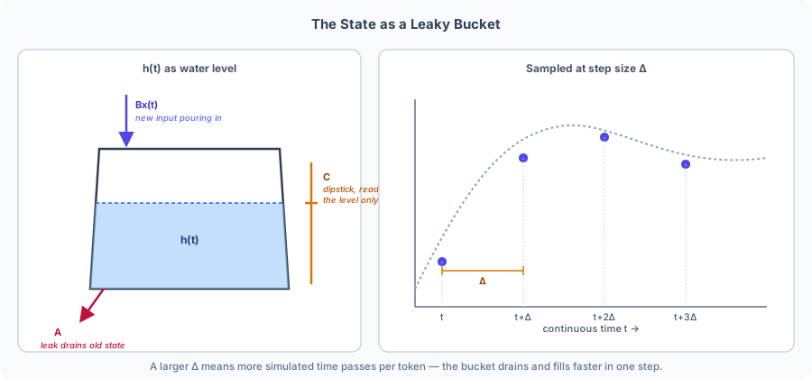
Diagram of a state space model as a leaky bucket: input pouring in as Bx(t), a leak at rate A, and a dipstick reading C, alongside a plot of the continuous state discretized at fixed step size Delta — Figure 4. The hidden state h(t) as a bucket of water: Bx(t) pours new input in, A is a leak draining old state away, and C is a dipstick reading the level without changing it. Discretization samples that continuous curve at a step size of Delta.

The bucket picture still holds: a larger $Δ$ means more simulated time passes per token, so $\overset{ˉ}{A}$ (how much of the old water level survives) shrinks toward zero and $\overset{ˉ}{B}$ (how much of the new input gets poured in) grows — the bucket both drains faster and fills faster over one step. A tiny $Δ$ does the opposite: $\overset{ˉ}{A} \approx I$ and $\overset{ˉ}{B} \approx 0$ , so almost nothing happens in that step at all. Hold onto that — it's the entire mechanism The Selection Mechanism builds on, three sections from now.

Equation (2) might look reverse-engineered to produce exactly this small- $Δ$ behavior. It isn't — it's the exact solution of Equation (1) under one very standard assumption, using a technique (zero-order hold) that's decades older than state space models and comes straight from classical control theory. That derivation is a detour from the main thread of this post, so it's worked out in full — every step, nothing skipped — in the appendix at the end, for anyone who wants to see it.

2.3. Discrete recurrence, and a worked example

Once discretized, the model runs exactly like an RNN — one step, one token, no differential equations left to solve:

h_{t} = \overset{ˉ}{A} h_{t - 1} + \overset{ˉ}{B} x_{t}, y_{t} = C h_{t} + D x_{t} (3)

To make this concrete, reuse the Transformer post's own toy sentence, "I think I understand" — the same four tokens, with "I" appearing twice, at positions 1 and 3. Here each token is reduced to a single scalar "signal" $x_{t}$ (state dimension $N = 2$ , model dimension $D = 1$ , so there's only one channel to track and no per-channel indexing to carry around — this $D$ is the model's channel count, the same overloaded use of the letter the Mamba paper itself makes; it has nothing to do with the feedthrough matrix $D$ from Equation (1), which Section 2.1 already set to zero for every example in this post), and $A$ is a fixed $2 \times 2$ diagonal matrix, written as just its two diagonal entries:

import numpy as np

def discretize(A, B, Delta):
    Abar = np.exp(Delta * A)
    Bbar = (Abar - 1.0) / A * B   # (Delta*A)^-1 (exp(Delta*A) - I) * Delta  ==  (Abar-1)/A
    return Abar, Bbar

tokens = ["I", "think", "I", "understand"]
x = np.array([-1.0, 0.5, -1.0, 1.0])

A = np.array([-1.0, -0.5])       # diagonal entries, fixed for the whole sequence
B, C, Delta = np.array([0.4, 0.4]), np.array([0.4, 0.4]), 1.0   # also fixed
D = 0.0   # the feedthrough matrix from equation 1/3, not the model dimension -- see Section 2.1

Abar, Bbar = discretize(A, B, Delta)
print("Abar", np.round(Abar, 3), "Bbar", np.round(Bbar, 3))
# Abar [0.368 0.607] Bbar [0.253 0.315]

h = np.zeros(2)
for tok, xt in zip(tokens, x):
    h = Abar * h + Bbar * xt
    y = C @ h + D * xt   # D = 0.0 throughout this post -- see Section 2.1
    print(f"{tok:10s} h={np.round(h, 3)}  y={round(float(y), 3)}")
# I          h=[-0.253 -0.315]  y=-0.227
# think      h=[ 0.033 -0.034]  y=-0.0
# I          h=[-0.241 -0.335]  y=-0.23
# understand h=[ 0.164  0.112]  y=0.11

$\overset{ˉ}{A}$ and $\overset{ˉ}{B}$ are computed once, from Equation (2), and then reused unchanged at every one of the four steps — that single fact, that the same two numbers apply no matter which word just came in, is exactly what Why Fixed Parameters Can't Selectively Remember comes back to break.

3. Two Views of the Same Computation

3.1. Unrolling the recurrence into a convolution

Because Equation (3) is linear, it can be unrolled by hand, one substitution at a time, starting from $h_{- 1} = 0$ (the same zero starting state every worked example in this post uses) and dropping the $D x_{t}$ term, since Section 2.1 already set $D = 0$ for the rest of this post — it would otherwise appear here as one more additive term, entirely outside the recurrence, since it never touches $h_{t}$ in the first place.

Step 1: unroll the state. Substitute Equation (3)'s own recurrence into itself — replace $h_{t - 1}$ with $\overset{ˉ}{A} h_{t - 2} + \overset{ˉ}{B} x_{t - 1}$ , then replace that $h_{t - 2}$ the same way, and so on, all the way back to $h_{- 1} = 0$ :

h_{t} = \overset{ˉ}{A} h_{t - 1} + \overset{ˉ}{B} x_{t} = \overset{ˉ}{A} (\overset{ˉ}{A} h_{t - 2} + \overset{ˉ}{B} x_{t - 1}) + \overset{ˉ}{B} x_{t} = \overset{ˉ}{A}^{2} h_{t - 2} + \overset{ˉ}{A} \overset{ˉ}{B} x_{t - 1} + \overset{ˉ}{B} x_{t} = \overset{ˉ}{A}^{2} (\overset{ˉ}{A} h_{t - 3} + \overset{ˉ}{B} x_{t - 2}) + \overset{ˉ}{A} \overset{ˉ}{B} x_{t - 1} + \overset{ˉ}{B} x_{t} = \overset{ˉ}{A}^{3} h_{t - 3} + \overset{ˉ}{A}^{2} \overset{ˉ}{B} x_{t - 2} + \overset{ˉ}{A} \overset{ˉ}{B} x_{t - 1} + \overset{ˉ}{B} x_{t} ⋮ = \overset{ˉ}{B} x_{t} + \overset{ˉ}{A} \overset{ˉ}{B} x_{t - 1} + \overset{ˉ}{A}^{2} \overset{ˉ}{B} x_{t - 2} + \dots (the leading \overset{ˉ}{A}^{t + 1} h_{- 1} term is always 0)

Step 2: read it out through $C$ . Apply Equation (3)'s own output equation, $y_{t} = C h_{t}$ (with $D = 0$ ), to the unrolled $h_{t}$ from step 1 — every term of the sum just picks up a $C$ in front:

y_{t} = C \overset{ˉ}{B} x_{t} + C \overset{ˉ}{A} \overset{ˉ}{B} x_{t - 1} + C \overset{ˉ}{A}^{2} \overset{ˉ}{B} x_{t - 2} + \dots (4)

Every $y_{t}$ in Equation (4) is a weighted sum over a window of past inputs, not just $x_{t}$ alone — and the weights $C \overset{ˉ}{B}, C \overset{ˉ}{A} \overset{ˉ}{B}, C \overset{ˉ}{A}^{2} \overset{ˉ}{B}, \dots$ never depend on $t$ , only on how many steps back you're looking. So the same short list of weights applies at every position, just slid over by one step each time $t$ increases by one: $C \overset{ˉ}{B}$ always multiplies whichever token is current, $C \overset{ˉ}{A} \overset{ˉ}{B}$ always multiplies whichever token came one step before it, and so on, regardless of which actual tokens those happen to be. Sliding one fixed list of weights along a sequence and reading off a weighted sum of whatever currently falls under it is the literal definition of a (1D, causal) convolution — the same operation a CNN's kernel performs sliding across an image, just sliding along time here instead of space. Collect those weights into one vector, call it $\overset{ˉ}{K}$ , and equation (4) becomes:

\overset{ˉ}{K} = (C \overset{ˉ}{B}, C \overset{ˉ}{A} \overset{ˉ}{B}, \dots, C \overset{ˉ}{A}^{L - 1} \overset{ˉ}{B}), y = x * \overset{ˉ}{K} (5)

To see the sliding actually happen, reuse Section 2.3's own numbers — $\overset{ˉ}{A} = [0.368, 0.607]$ , $\overset{ˉ}{B} = [0.253, 0.315]$ , $C = [0.4, 0.4]$ — and collapse the two state channels the same way $C \overset{ˉ}{A}^{i} \overset{ˉ}{B}$ does at each offset $i$ , giving four fixed kernel taps that hold for the whole sequence:

\overset{ˉ}{K}_{0} \approx 0.227, \overset{ˉ}{K}_{1} \approx 0.114, \overset{ˉ}{K}_{2} \approx 0.060, \overset{ˉ}{K}_{3} \approx 0.033

Sliding $\overset{ˉ}{K}$ under $x = (- 1.0, 0.5, - 1.0, 1.0)$ ("I", "think", "I", "understand") so that $\overset{ˉ}{K}_{0}$ always lines up with the current token, $\overset{ˉ}{K}_{1}$ with one token back, $\overset{ˉ}{K}_{2}$ with two back, and so on, gives:

y_{1} y_{2} y_{3} y_{4} = \overset{ˉ}{K}_{0} x_{1} \approx - 0.227 = \overset{ˉ}{K}_{0} x_{2} + \overset{ˉ}{K}_{1} x_{1} \approx - 0.000 = \overset{ˉ}{K}_{0} x_{3} + \overset{ˉ}{K}_{1} x_{2} + \overset{ˉ}{K}_{2} x_{1} \approx - 0.230 = \overset{ˉ}{K}_{0} x_{4} + \overset{ˉ}{K}_{1} x_{3} + \overset{ˉ}{K}_{2} x_{2} + \overset{ˉ}{K}_{3} x_{1} \approx 0.110

the exact same four numbers Section 2.3's recurrence printed, one token at a time. Notice that $\overset{ˉ}{K}_{0}, \dots, \overset{ˉ}{K}_{3}$ never changed across those four sums — only which $x$ each one lined up with changed, sliding over by one position every step. That's exactly what a convolution kernel does: the same fixed weights, run over a shifting window of the input.

3.2. Training as convolution, generating as recurrence

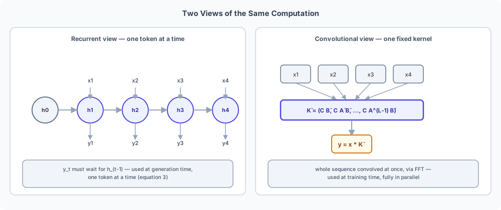
Side-by-side diagram of the recurrent view of a state space model (a chain of hidden states updated one token at a time) and the convolutional view (a fixed kernel slid over the whole input sequence at once) — Figure 5. The same linear recurrence, unrolled two ways: as a chain of steps (used one token at a time during generation) or as one fixed convolution kernel applied to the whole sequence at once (used during training, for full parallelism).

This dual view is the whole reason pre-Mamba state space models like S4 [2] were fast to train in the first place.

Precompute $\overset{ˉ}{K}$ once, from $\overset{ˉ}{A}, \overset{ˉ}{B}, C$ alone. Every tap $\overset{ˉ}{K}_{i} = C \overset{ˉ}{A}^{i} \overset{ˉ}{B}$ involves only the model's fixed parameters, never the actual input $x$ — so it can be worked out up front, with no data in sight. $\overset{ˉ}{K}_{i}$ is the answer to "if one unit of input had arrived $i$ steps ago and decayed through $\overset{ˉ}{A}$ ever since, how much of it would $C$ still read off today?" That's the system's impulse response, and it's the whole reason Section 3.1's kernel is a fixed list of numbers in the first place, computable before a single real token shows up.

Training: skip $h$ entirely, and do every position at once. Once $\overset{ˉ}{K}$ exists, $y_{t} = \sum_{i} \overset{ˉ}{K}_{i} x_{t - i}$ reads straight off the raw inputs — $h_{t}$ never gets built at all. Convolving $\overset{ˉ}{K}$ against the whole sequence the naive way — sliding it one step at a time, the way Section 3.1's four sums did by hand — costs $O (L^{2})$ . A convolution is exactly the computation the Fast Fourier Transform (FFT) is built to speed up: a decades-old algorithm, unrelated to state space models, that computes the same result in $O (L lo g L)$ without sliding step by step at all. Either way, $y_{1}, y_{2}, y_{3}, \dots$ are independent sums over data that's already all there during training, so every one of them can be computed simultaneously — no waiting for $h_{t - 1}$ to materialize before $y_{t}$ , the exact problem RNNs have.

Generation: no future to convolve over, so it's an RNN again. Tokens now arrive one at a time, and there's no "whole sequence" yet to slide $\overset{ˉ}{K}$ across — tomorrow's tokens don't exist yet. So the same model switches to Equation (3)'s recurrent form instead, exactly like an RNN, with the same $O (1)$ -per-step, constant-memory inference Pick Two: Parallelism, Speed, or Memory promised. Same $\overset{ˉ}{A}$ , $\overset{ˉ}{B}$ , $C$ ; two different ways of running the arithmetic, picked for whichever situation — training on a fixed sequence, or generating one token at a time — you're actually in.

4. Why Fixed Parameters Can't Selectively Remember

Section 1.2 ended on a promise: build a recurrence competitive with attention's quality, not just its speed. Attention gets that quality by looking back over every previous token at each step and weighting them by content — a filler word and the key noun get different weights, regardless of distance. It can do this because it never compresses: every past token's key and value is kept, which is exactly the growing cache Section 9.1 measures. That per-token, content-based weighting is what "selectively remember" means here.

A recurrence works the opposite way: it never keeps individual tokens, only one fixed-size state $h_{t}$ , updated as each token arrives. Whatever the update doesn't capture is lost. That's what makes it cheap — but it means the update itself has to do attention's job: decide, per token, how much to keep. 4.1 shows that with $\overset{ˉ}{A}, \overset{ˉ}{B}$ fixed, it can't.

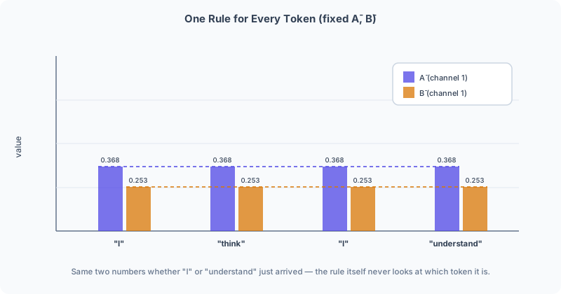
4.1. One rule for every token

Go back to the worked example in Discrete recurrence, and a worked example. $\overset{ˉ}{A}$ and $\overset{ˉ}{B}$ came out to [0.368 0.607] and [0.253 0.315] — and stayed exactly those two numbers at "I", at "think", and at "understand". The model has no way to look at $x_{t}$ and decide "this one matters more" or "this one's just a filler word, don't bother updating the state much" — the update rule is identical no matter what token just arrived, because $\overset{ˉ}{A}$ and $\overset{ˉ}{B}$ are constants set before the sequence is even seen.

Bar chart showing Abar and Bbar staying identical across four different tokens in a fixed-parameter, linear time-invariant state space model — Figure 6. In a fixed-parameter (LTI) state space model, Abar and Bbar are the same two numbers no matter which token just arrived — a filler word and a content word update the state by exactly the same rule.

4.2. Where this actually breaks: selective copying

This isn't hypothetical. The Mamba paper tests it directly with a synthetic benchmark, selective copying: most tokens are blank filler, a few are real content, and the task is to reproduce just the content, in order, ignoring the filler. Unlike "I" in the sentence example, which still carries some signal, these filler tokens carry none — the contrast is total. Solving this requires the recurrence to decide, per token, whether to write to memory at all: barely touch it for filler, write firmly for content.

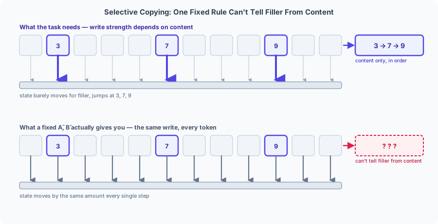
Figure 7. Selective copying needs the write strength into the state to depend on content — barely touching it for filler, writing firmly for the content tokens 3, 7, and 9 — so the output can be just the content, in order. A fixed Ā, B̄ writes by the same amount every single step, so it can't tell filler from content in the first place. (Digits, not letters, stand in for content here so they stay distinct from the A, B, C matrices used everywhere else in this post.)

A fixed $\overset{ˉ}{A}, \overset{ˉ}{B}$ can't make that decision, because the decision requires looking at the content of $x_{t}$ , and fixed parameters are chosen before the model ever sees the input.

A system with a constant $A$ , $B$ , $C$ is called linear time-invariant (LTI) — "time-invariant" meaning the rule itself is the same at every position, regardless of position or content. LTI is exactly what makes the convolution view possible: a fixed kernel $\overset{ˉ}{K}$ only makes sense if the same weights genuinely apply at every offset. Section 6 comes back to this trade directly — selectivity and the convolution view turn out to be mutually exclusive.

5. The Selection Mechanism: Let the Input Set the Dials

5.1. Three small projections, read off the input

$Δ$ isn't one of the original state-space matrices — it's the step size from Discretization: turning a rate into a step. Equation (2) already showed what it does: a large $Δ$ drains $\overset{ˉ}{A}$ toward zero and grows $\overset{ˉ}{B}$ , so the old state drains away and the current token dominates; a tiny $Δ$ leaves $\overset{ˉ}{A} \approx I$ and $\overset{ˉ}{B} \approx 0$ , so almost nothing happens. That's the write-time lever Section 4 was missing — it just needs to depend on the token instead of staying fixed. $B$ and $C$ are simpler: $B$ controls how much of the input enters the state, $C$ controls how much of the state reaches the output. Mamba makes all three functions of the current token $x_{t}$ , computed fresh at every step:

B_{t} C_{t} Δ_{t} = s_{B} (x_{t}) = W_{B} x_{t} = s_{C} (x_{t}) = W_{C} x_{t} = softplus (b_{Δ} + w_{Δ} x_{t}) (6)

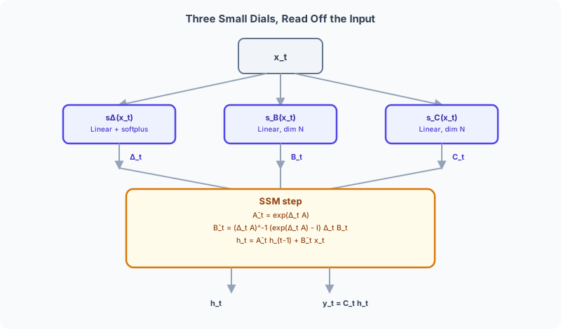
Figure 8. Three small linear projections read the current token and produce Delta_t, B_t, and C_t fresh at every step, instead of reusing the same three constants the whole sequence through.

$A$ itself stays fixed — it's still initialized once, the way HiPPO [3] theory prescribes for S4-style models — but $Δ_{t}$ feeds into $\overset{ˉ}{A}_{t} = exp (Δ_{t} A)$ from Equation (2), so the discretized $\overset{ˉ}{A}_{t}$ ends up input-dependent anyway, indirectly, through $Δ_{t}$ . softplus — $softplus (z) = ln (1 + e^{z})$ — just keeps $Δ_{t}$ strictly positive, the way a step size has to be, while still letting $w_{Δ} x_{t}$ push it arbitrarily large or small.

5.2. Δ as a gate

The bucket metaphor from The continuous equations, and a bucket to picture them with explains exactly what a selective $Δ_{t}$ buys: a small $Δ_{t}$ means $\overset{ˉ}{A}_{t} \approx I$ and $\overset{ˉ}{B}_{t} \approx 0$ (Equation (2)) — almost none of this token gets poured in, and almost all of the old water level survives untouched. A large $Δ_{t}$ does the opposite — $\overset{ˉ}{A}_{t}$ shrinks toward zero and $\overset{ˉ}{B}_{t}$ grows, so the old state mostly drains away and the new token dominates what's left. $Δ_{t}$ is, in effect, a per-token gate deciding "skip this" versus "reset around this" — precisely the decision a fixed $\overset{ˉ}{A}, \overset{ˉ}{B}$ could never make.

5.3. Worked example: the same four tokens, now selective

Assign each token in "I think I understand" a scalar $x_{t}$ chosen so "I" reads as a filler and "understand" reads as the sentence's actual content — the same values used in Discrete recurrence, and a worked example's STATIC run, run again through Equation (6) instead of fixed constants:

def softplus(z):
    return np.log1p(np.exp(z))

w_B, w_C, w_delta, b_delta = np.array([0.4, 0.4]), np.array([0.4, 0.4]), 2.0, 0.0

h = np.zeros(2)
for tok, xt in zip(tokens, x):
    Delta_t = softplus(w_delta * xt + b_delta)
    B_t, C_t = w_B * xt, w_C * xt
    Abar_t, Bbar_t = discretize(A, B_t, Delta_t)
    h_prev = h.copy()
    h = Abar_t * h + Bbar_t * xt
    y = C_t @ h + D * xt   # D is still 0.0, reused unchanged from the STATIC example above
    print(f"{tok:10s} Delta={Delta_t:.3f}  Abar={np.round(Abar_t, 3)}  "
          f"h_prev={np.round(h_prev, 3)} -> h={np.round(h, 3)}  y={round(float(y), 3)}")
# I          Delta=0.127  Abar=[0.881 0.939]  h_prev=[0. 0.]         -> h=[0.048 0.049]  y=-0.039
# think      Delta=1.313  Abar=[0.269 0.519]  h_prev=[0.048 0.049]   -> h=[0.086 0.122]  y=0.042
# I          Delta=0.127  Abar=[0.881 0.939]  h_prev=[0.086 0.122]   -> h=[0.123 0.163]  y=-0.115
# understand Delta=2.127  Abar=[0.119 0.345]  h_prev=[0.123 0.163]   -> h=[0.367 0.58 ]  y=0.379

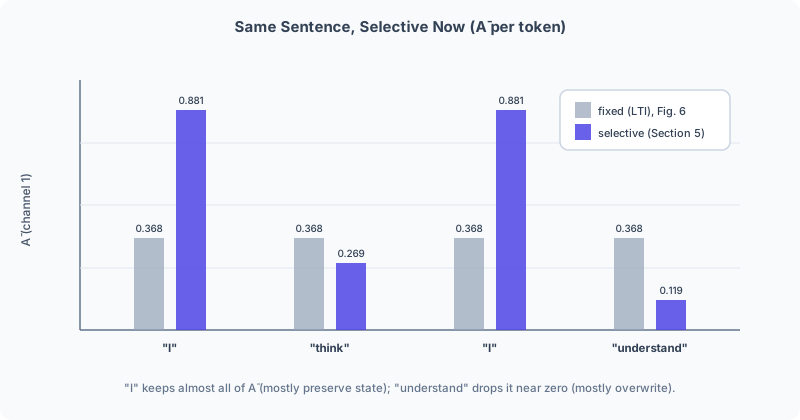
Δ_{I} = 0.127, Δ_{think} = 1.313, Δ_{I} = 0.127, Δ_{understand} = 2.127 (7)

Grouped bar chart comparing constant Abar values across four tokens against varying, input-dependent Abar values for the same four tokens under the selection mechanism — Figure 9. The same four tokens as Figure 6, now with Abar varying per token: near 1 at the filler word "I" (mostly preserve old state), and much smaller at the content word "understand" (mostly overwrite it).

Compare the two "I" rows against the "understand" row: at "I", $\overset{ˉ}{A}_{t}$ sits near [0.88, 0.94] — almost all of $h_{prev}$ survives, and $h$ barely moves ([0.086 0.122] to [0.123 0.163], a small nudge). At "understand", $\overset{ˉ}{A}_{t}$ drops to [0.12, 0.35] — most of the old state drains away — and $h$ jumps ([0.123 0.163] to [0.367 0.58], roughly triple). Nothing in the STATIC run could ever produce that contrast, because $\overset{ˉ}{A}$ and $\overset{ˉ}{B}$ there were the same two numbers at every single token, filler or not.

6. The Price of Selection: No More Convolution

Two Views of the Same Computation's convolution kernel $\overset{ˉ}{K} = (C \overset{ˉ}{B}, C \overset{ˉ}{A} \overset{ˉ}{B}, \dots)$ only makes sense if $\overset{ˉ}{A}$ and $\overset{ˉ}{B}$ are the same matrices at every offset — that's what let a single kernel, computed once, apply uniformly across the whole sequence. The moment $\overset{ˉ}{A}_{t}$ and $\overset{ˉ}{B}_{t}$ change at every $t$ , as Equation (6) makes them, there is no longer one kernel to compute — there'd need to be a different kernel at every position, which isn't a convolution at all anymore. Selectivity buys exactly the thing Why Fixed Parameters Can't Selectively Remember was missing, but it costs the FFT-parallel training trick that made LTI state space models fast, seemingly forcing a return to the RNN's one-step-at-a-time training. Section 7 is Mamba's answer to that trade-off.

7. Parallel Scan: Getting Parallelism Back

7.1. An operator that composes affine steps

Equation (3)'s recurrence, $h_{t} = \overset{ˉ}{A}_{t} h_{t - 1} + \overset{ˉ}{B}_{t} x_{t}$ , is an affine map applied to $h_{t - 1}$ at every step: write it as $h_{t} = a_{t} h_{t - 1} + b_{t}$ , with $a_{t}$ standing for $\overset{ˉ}{A}_{t}$ and $b_{t}$ for $\overset{ˉ}{B}_{t} x_{t}$ . Chain two consecutive steps, $i$ then $j$ , by substituting the first directly into the second:

h_{j} = a_{j} h_{i} + b_{j} = a_{j} (a_{i} h_{i - 1} + b_{i}) + b_{j} = (a_{i} a_{j}) h_{i - 1} + (a_{j} b_{i} + b_{j})

Whatever $h_{i - 1}$ turns out to be, running step $i$ then step $j$ is identical to running one combined step with slope $a_{i} a_{j}$ and intercept $a_{j} b_{i} + b_{j}$ — and neither of those two numbers involves $h_{i - 1}$ at all. $a_{j} b_{i}$ isn't two different tokens' $B$ getting mixed together; by the time step $j$ runs, $b_{i}$ is just a fixed number already sitting in $h_{i}$ , and $a_{j}$ decays it the same way the bucket drains whatever it's already holding. Collect the two combined numbers into a pair, and this substitution is the combine operator:

(a_{i}, b_{i}) ∙ (a_{j}, b_{j}) = (a_{i} a_{j}, a_{j} b_{i} + b_{j}) (8)

Because ordinary multiplication and addition are associative, $∙$ is too: $(P ∙ Q) ∙ R$ gives the same pair as $P ∙ (Q ∙ R)$ . That's the one property a parallel scan (or prefix-sum) algorithm needs: an associative operator can be applied to disjoint chunks of a sequence independently, then those chunk-results combined afterward, rather than folding strictly left to right — and since $∙$ never touches $h$ , two far-apart steps can be combined before either one ever sees the actual running state.

7.2. Worked example: four steps in two rounds

Take the four (Abar, Bbar·x) pairs from Worked example: the same four tokens, now selective — tracking just the first of the two state channels, to keep the arithmetic on one line — and combine them pairwise instead of one at a time:

def combine(P, Q):
    aP, bP = P
    aQ, bQ = Q
    return (aP * aQ, aQ * bP + bQ)

# (Abar[0], Bbar[0]*x) for I, think, I, understand -- channel 0 only, from section 5.3.
# Bbar[0] for "I" is -0.048, but x is -1.0 there too, so Bbar[0]*x = +0.048.
steps = [(0.881, 0.048), (0.269, 0.073), (0.881, 0.048), (0.119, 0.352)]

P12 = combine(steps[0], steps[1])
P34 = combine(steps[2], steps[3])
P14 = combine(P12, P34)
print("P12", np.round(P12, 3), "P34", np.round(P34, 3), "P14", np.round(P14, 3))
# P12 [0.237 0.086] P34 [0.105 0.358] P14 [0.025 0.367]

h4 = P14[0] * 0.0 + P14[1]     # h_{-1} = 0
print(round(h4, 3))
# 0.367

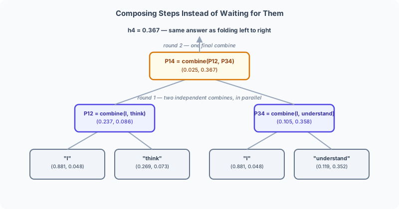
Tree diagram showing four sequential recurrence steps combined pairwise into two intermediate results, then combined once more into a single final result — Figure 10. Four steps combined in two rounds instead of four: adjacent pairs combine independently first, then the two intermediate results combine once more — the same final answer as folding strictly left to right, reached in log(L) rounds instead of L.

0.367 is exactly the first entry of h after "understand" in the selective worked example — computed here without ever folding left to right through all four steps in sequence. P12 and P34 can be computed at the same time, since neither depends on the other, and only the final combine(P12, P34) waits on both — two sequential "rounds" for four tokens instead of four, and for $L$ tokens this generalizes to $O (lo g L)$ rounds instead of $O (L)$ .

7.3. Hardware-aware: why this still needs custom kernels

The algorithm above is parallel on paper, but naively materializing every intermediate $(\overset{ˉ}{A}_{t}, \overset{ˉ}{B}_{t})$ pair for every channel and every batch element is a lot of memory traffic — the actual Mamba implementation fuses discretization, the scan, and the final elementwise multiply into a single GPU kernel that keeps intermediate values in fast on-chip SRAM and only writes the final output back to slower HBM, an optimization in the same spirit as FlashAttention's approach to fusing attention's own intermediate steps. None of that changes the math in Equation (8) — it changes only how cheaply a GPU can execute it.

8. The Mamba Block: Assembling the Layer

8.1. Expand, branch, gate, project

Everything so far — discretization, selection, the scan — lives inside a single sub-block called the selective SSM (SSM: state space model, the machinery built in Sections 2-7). A full Mamba block wraps that sub-block the same way a Transformer block wraps self-attention: a linear projection first, the core computation in the middle, a linear projection back out, all inside a residual connection.

u, z u^{'} y o = split (Linear_{in} (u_{0})) = SiLU (Conv1d (u)) = SSM_{Δ, B, C} (u^{'}) = Linear_{out} (y ⊙ SiLU (z)) (9)

Architecture diagram of a Mamba block: an input projection splitting into a convolution-SiLU-SSM branch and a SiLU gating branch, multiplied together, then projected back out, inside a residual connection — Figure 11. One Mamba block: the input is projected up and split in two. One branch runs a short causal convolution, SiLU, then the selective SSM; the other is a pure SiLU gate. Their elementwise product is projected back down and added back via a residual connection.

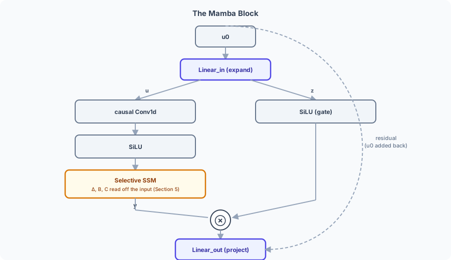
The input $u_{0}$ is projected up to a wider dimension and split into two branches. The first branch $u$ goes through a small causal depthwise convolution — a short local look-back, mixing each position with the handful just before it, before the SSM ever sees it — then a SiLU nonlinearity ( $SiLU (x) = x \cdot σ (x)$ , a smooth alternative to ReLU that lets small negative values through instead of zeroing them), then the selective SSM itself, exactly as derived in The Selection Mechanism. The second branch $z$ is a pure gate: SiLU applied to a separate linear projection of the same input, with no SSM in it at all. The two branches meet only at $y ⊙ SiLU (z)$ , an elementwise product — the gate branch gets to scale down or shut off individual channels of the SSM's output before the final projection brings the dimension back down to $u_{0}$ 's size. This design — a convolution-then-SSM branch multiplicatively gated by a second branch — comes from H3 [4], folded together with a standard gated-MLP block; Mamba's own contribution on top is entirely inside the "SSM" box, not the branching structure around it.

8.2. Where this sits in a full model

A full Mamba model is a stack of these blocks, each one wrapped in the same pre-norm-plus-residual pattern a Transformer block uses — a normalization layer, then the block, then added back to its own input — repeated some number of layers deep, with an embedding table at the bottom and a vocabulary projection at the top, exactly like the decoder post's own architecture. The only thing that changes, layer to layer, is what sits between the two residual connections: self-attention there, this block here.

9. What Mamba Buys You, and What It Costs

9.1. A state that never grows

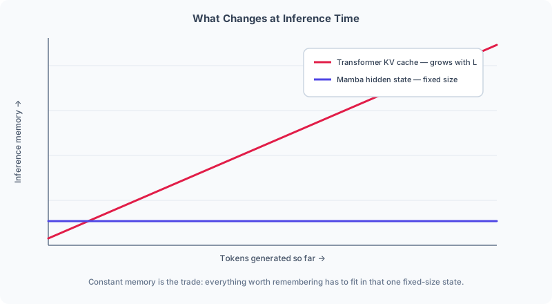
Line plot of inference memory against sequence length, showing a growing Transformer key/value cache against Mamba's constant-size hidden state — Figure 12. A Transformer's key/value cache grows with every generated token. Mamba's inference state is a single fixed-size hidden vector, the same size at token 10 as at token 10,000 — the trade-off is that it has to compress everything worth remembering into that fixed size, rather than keeping perfect memory of every past token.

The decoder post's causal masking section already established why generating the $t$ -th token with a Transformer means keeping every previous position's key and value vectors around — a cache that grows linearly with how much has been generated so far, and gets attended to in full at every subsequent step. Mamba's inference state is the hidden vector $h_{t}$ from Equation (3), alone — a fixed size, set by the state dimension $N$ , that never grows no matter how long the sequence gets. Generating token 10,000 costs exactly what generating token 10 cost, an actual $O (1)$ -per-step guarantee Pick Two: Parallelism, Speed, or Memory opened this post with.

9.2. Where attention still wins

That fixed-size state is also the honest limitation: a Transformer's KV cache is, in effect, perfect memory — token 10,000 can attend directly back to token 1's exact key and value, no matter how much has happened in between. Mamba's $h_{t}$ has to compress everything worth remembering into one $N$ -dimensional vector, and $N$ doesn't grow with the sequence. Tasks that need exact long-range recall — repeating back a specific token from thousands of positions ago, verbatim — are precisely where a fixed-size state is most likely to have already overwritten what it needed. This is an active area past the original paper: Mamba-2 [5] reframes the selective SSM as a form of linear attention to close part of that gap, and several hybrid architectures interleave ordinary attention layers with SSM layers rather than picking one mechanism for an entire model — betting that a few layers of perfect, expensive memory plus many layers of cheap, approximate memory beats either extreme alone.

10. Putting It All Together

10.1. Discretize and scan

The two functions this whole post is really about — both already exhaustively worked by hand above — as plain, runnable NumPy:

import numpy as np

def softplus(z):
    return np.log1p(np.exp(z))

def discretize(A, B, Delta):
    """Zero-order hold, equation 2. A: (N,) diagonal entries. B: (N,). Delta: scalar."""
    Abar = np.exp(Delta * A)
    Bbar = (Abar - 1.0) / A * B
    return Abar, Bbar

def selective_ssm_step(h_prev, x_t, A, W_B, W_C, w_delta, b_delta, D):
    """One selective-SSM step (equations 3 and 6). h_prev, A, W_B, W_C: (N,). x_t, w_delta,
    b_delta, D: scalars, since this reference sticks to one channel throughout. D here is
    equation 1/3's feedthrough matrix, not the model-dimension D used elsewhere in this post's
    prose -- pass D=0.0 to match every worked example above (Section 2.1). Returns the new
    hidden state and this step's output."""
    Delta_t = softplus(w_delta * x_t + b_delta)
    B_t, C_t = W_B * x_t, W_C * x_t
    Abar_t, Bbar_t = discretize(A, B_t, Delta_t)
    h_t = Abar_t * h_prev + Bbar_t * x_t
    y_t = C_t @ h_t + D * x_t
    return h_t, y_t

def selective_scan(x, A, W_B, W_C, w_delta, b_delta, D):
    """Sequential reference scan (Section 5.3's worked loop, generalized). A real
    implementation replaces this loop with the parallel-scan/combine of Section 7, computed
    inside a fused GPU kernel -- the output is identical either way."""
    h = np.zeros_like(A)
    ys = []
    for x_t in x:
        h, y_t = selective_ssm_step(h, x_t, A, W_B, W_C, w_delta, b_delta, D)
        ys.append(y_t)
    return np.array(ys)

10.2. The Mamba block

Section 8's branching structure (Equation (9)), with the selective SSM above as its core:

def silu(z):
    return z / (1.0 + np.exp(-z))

def causal_conv1d(u, kernel):
    """Depthwise causal convolution: position t only ever sees positions <= t. kernel: a short
    per-channel filter, applied independently to each channel of u."""
    L = len(u)
    k = len(kernel)
    padded = np.concatenate([np.zeros(k - 1), u])   # left-pad so output length stays L
    return np.array([np.dot(padded[t:t + k], kernel) for t in range(L)])

def mamba_block(u0, W_in, conv_kernel, A, W_B, W_C, w_delta, b_delta, D, W_out):
    """u0: (L,) input sequence, one scalar channel, matching this post's worked examples.
    W_in projects to two branches; W_out projects the gated result back down (equation 9)."""
    projected = u0 * W_in            # (L, 2) -- toy stand-in for Linear_in
    u, z = projected[:, 0], projected[:, 1]

    u_conv = causal_conv1d(u, conv_kernel)
    u_prime = silu(u_conv)

    y = selective_scan(u_prime, A, W_B, W_C, w_delta, b_delta, D)

    gated = y * silu(z)
    return gated * W_out              # toy stand-in for Linear_out

causal_conv1d and the two toy W_in/W_out stand-ins are simplified to a single scalar channel throughout, matching every worked example in this post's model dimension of 1; a real Mamba layer runs this same logic independently across however many channels the model's expanded inner dimension has, and selective_scan's sequential Python loop is exactly what Parallel Scan's combine operator replaces on real hardware — different order of operations, identical numbers out.

Appendix: Where Equation 2 Actually Comes From

Discretization: turning a rate into a step stated Equation (2) without deriving it, and promised that the small- $Δ$ behavior it produces — $\overset{ˉ}{A} \to I$ , $\overset{ˉ}{B} \to 0$ — isn't a designed-in limit but a mathematical consequence of exactly solving Equation (1). This appendix makes good on that promise, spelling out every step of the derivation, including the two calculus facts it leans on (how to differentiate a matrix exponential, and the product rule) rather than assuming them.

The setup. Zero-order hold assumes the input $x (t)$ is held constant at $x_{t}$ for one whole step (that's the "hold" in the name — the simplest way to turn one discrete sample into a continuous signal is to hold it flat until the next sample arrives). Re-anchor time so that step runs from $τ = 0$ to $τ = Δ$ , with $h (0) = h_{t - 1}$ . Equation (1)'s state equation, with $x (t)$ now a fixed constant $x_{t}$ instead of a function of time, becomes an ordinary linear differential equation with constant forcing:

h^{'} (τ) = A h (τ) + B x_{t}, h (0) = h_{t - 1}

A refresher: differentiating the matrix exponential. The rest of this derivation leans on one calculus fact: $\frac{d}{d τ} e^{X τ} = X e^{X τ}$ , for any fixed matrix $X$ . This isn't special to matrices — it's true for exactly the same reason $\frac{d}{d τ} e^{a τ} = a e^{a τ}$ is true for a plain number $a$ , because $e^{X τ}$ is defined by the same power series as the scalar exponential, just with $X τ$ in place of a number:

e^{X τ} = I + X τ + \frac{( X τ ) ^{2}}{2 !} + \frac{( X τ ) ^{3}}{3 !} + \dots

Differentiating term by term with respect to $τ$ (each term is just $τ$ raised to a power, times a constant matrix, so ordinary single-variable calculus applies to each one separately):

\frac{d}{d τ} e^{X τ} = X + X^{2} τ + \frac{X ^{3} τ ^{2}}{2 !} + \dots = X (I + X τ + \frac{( X τ ) ^{2}}{2 !} + \dots) = X e^{X τ}

Setting $X = - A$ gives the specific fact this derivation needs: $\frac{d}{d τ} e^{- A τ} = - A e^{- A τ}$ .

The product rule, spelled out. For two ordinary functions $f (τ)$ and $g (τ)$ , the product rule says $\frac{d}{d τ} [f (τ) g (τ)] = f^{'} (τ) g (τ) + f (τ) g^{'} (τ)$ — the same rule taught in any first calculus course. It holds just as well when $f (τ)$ is a matrix-valued function and $g (τ)$ is a vector-valued one, for the same reason the sum and constant-multiple rules carry over: differentiation is applied entry by entry, and every entry of $f (τ) g (τ)$ is an ordinary sum of products of scalar functions, each of which obeys the scalar product rule individually.

Apply it with $f (τ) = e^{- A τ}$ and $g (τ) = h (τ)$ , using $f^{'} (τ) = - A e^{- A τ}$ from the step above:

\frac{d}{d τ} [e^{- A τ} h (τ)] = f^{'} (τ) (- A e^{- A τ}) h (τ) + f (τ) e^{- A τ} g^{'} (τ) h^{'} (τ)

$A$ commutes with any power series built out of $A$ — including $e^{- A τ}$ , which is exactly such a series — so $- A e^{- A τ} h (τ)$ can be rewritten as $e^{- A τ} (- A h (τ))$ , and the two terms above factor together:

\frac{d}{d τ} [e^{- A τ} h (τ)] = e^{- A τ} (h^{'} (τ) - A h (τ))

The ODE from the setup says $h^{'} (τ) = A h (τ) + B x_{t}$ , i.e. $h^{'} (τ) - A h (τ) = B x_{t}$ . Substituting that in:

\frac{d}{d τ} [e^{- A τ} h (τ)] = e^{- A τ} B x_{t}

This is the entire point of multiplying by $e^{- A τ}$ in the first place (the classical "integrating factor" trick): it turns a differential equation that mixes $h (τ)$ and $h^{'} (τ)$ into a plain derivative of a single product, sitting on the left, with nothing but a function of $τ$ on the right — which can now just be integrated directly.

Integrating both sides. Integrate from $τ = 0$ to $τ = Δ$ . The left side is the derivative of something, so the fundamental theorem of calculus collapses it to the difference of its endpoint values:

\int_{0}^{Δ} \frac{d}{d τ} [e^{- A τ} h (τ)] d τ = e^{- A Δ} h (Δ) - e^{0} h (0) = e^{- A Δ} h (Δ) - h (0)

On the right, $x_{t}$ is constant over the step by assumption, so it factors outside the integral, leaving just the integral of a matrix exponential:

\int_{0}^{Δ} e^{- A τ} B x_{t} d τ = (\int_{0}^{Δ} e^{- A τ} d τ) B x_{t}

The integral of a matrix exponential. Claim: $\int e^{- A τ} d τ = - A^{- 1} e^{- A τ}$ . Check it the same way any antiderivative gets checked — differentiate it and confirm the original function comes back, using $\frac{d}{d τ} e^{- A τ} = - A e^{- A τ}$ from two steps ago:

\frac{d}{d τ} [- A^{- 1} e^{- A τ}] = - A^{- 1} (- A e^{- A τ}) = A^{- 1} A e^{- A τ} = e^{- A τ} ✓

So the claimed antiderivative is correct, and:

\int_{0}^{Δ} e^{- A τ} d τ = [- A^{- 1} e^{- A τ}]_{0}^{Δ} = - A^{- 1} e^{- A Δ} - (- A^{- 1} e^{0}) = A^{- 1} (I - e^{- A Δ})

Solving for $h (Δ)$ . Putting the left and right sides from "Integrating both sides" back together:

e^{- A Δ} h (Δ) - h (0) = A^{- 1} (I - e^{- A Δ}) B x_{t}

Multiply both sides by $e^{A Δ}$ (the inverse of $e^{- A Δ}$ , since $e^{A Δ} e^{- A Δ} = I$ for any matrix):

h (Δ) = e^{A Δ} h (0) + e^{A Δ} A^{- 1} (I - e^{- A Δ}) B x_{t}

Simplify the second term the same way as before — $A$ (and its inverse) commute with $e^{A Δ}$ :

e^{A Δ} A^{- 1} (I - e^{- A Δ}) = A^{- 1} e^{A Δ} (I - e^{- A Δ}) = A^{- 1} (e^{A Δ} - I)

giving:

h (Δ) = e^{A Δ} h (0) + A^{- 1} (e^{A Δ} - I) B x_{t}

That's Equation (2), exactly — $\overset{ˉ}{A} = e^{A Δ} = exp (Δ A)$ , and $\overset{ˉ}{B} = A^{- 1} (e^{Δ A} - I) B$ , the same thing as $(Δ A)^{- 1} (exp (Δ A) - I) Δ B$ once the $Δ$ 's are multiplied back in and canceled (kept explicit in that form since $Δ$ is about to become a learned, per-token parameter in The Selection Mechanism). Nothing in this derivation was chosen to produce a particular limit — every step above is either the definition of the matrix exponential, the ordinary product rule, or the fundamental theorem of calculus.

A concrete check. Plug in the toy $A = diag (- 1, - 0.5)$ and $B = [0.4, 0.4]$ — the same two values the worked example uses for its full recurrence — at $Δ = 1.0$ :

import numpy as np

A = np.array([-1.0, -0.5])
B = np.array([0.4, 0.4])

Abar = np.exp(1.0 * A)
Bbar = (Abar - 1.0) / A * B
print(np.round(Abar, 3), np.round(Bbar, 3))
# [0.368 0.607] [0.253 0.315]

That matches $\overset{ˉ}{A}$ and $\overset{ˉ}{B}$ exactly as the worked example computes them too, because it's the same formula being evaluated on the same numbers — the derivation above didn't introduce any new approximation on top of what equation 2 already says.

Why the small- $Δ$ limit isn't tuned. Expand $e^{Δ A}$ using the same power series introduced above, $e^{Δ A} = I + Δ A + \frac{1}{2} (Δ A)^{2} + \dots$ . As $Δ \to 0$ , every term past the first vanishes, so $\overset{ˉ}{A} = e^{Δ A} \to I$ — not because $\overset{ˉ}{A}$ was built to converge to $I$ , but because any convergent power series in $Δ$ reduces to its constant term as $Δ \to 0$ , and here the constant term happens to be $I$ . The same expansion, substituted into $\overset{ˉ}{B} = A^{- 1} (e^{Δ A} - I) B$ , gives $\overset{ˉ}{B} = A^{- 1} (Δ A + O (Δ^{2})) B = Δ B + O (Δ^{2})$ — so $\overset{ˉ}{B} \to 0$ linearly in $Δ$ , not because it was designed to shrink, but because that's what's left of the expansion once the constant term cancels against the $- I$ . Checking this numerically, at $Δ = 0.01$ against the same toy $A$ and $B$ :

Abar_tiny, Bbar_tiny = np.exp(0.01 * A), (np.exp(0.01 * A) - 1.0) / A * B
print(np.round(Abar_tiny, 5), np.round(Bbar_tiny, 5), np.round(0.01 * B, 5))
# [0.99005 0.99501] [0.00398 0.00399] [0.004 0.004]

$\overset{ˉ}{B}$ already sits within rounding error of $Δ B$ , exactly as the first-order Taylor term predicts. This is why the "gate" reading of $Δ$ isn't a second mechanism layered on top of discretization — it's a direct consequence of solving equation 1 exactly, one that would show up in any discretization built the same way. (S4's earlier variants also tried the bilinear/Tustin transform instead of zero-order hold; both satisfy the same small- $Δ$ limit, since that's a property every consistent discretization of an ODE has to have, not something specific to the zero-order-hold choice.)

References

[1]Gu & Dao (2023). Mamba: Linear-Time Sequence Modeling with Selective State Spaces.
[2]Gu, Goel & Ré (2021). Efficiently Modeling Long Sequences with Structured State Spaces. International Conference on Learning Representations (ICLR).
[3]Gu, Dao, Ermon, Rudra & Ré (2020). HiPPO: Recurrent Memory with Optimal Polynomial Projections. Neural Information Processing Systems (NeurIPS).
[4]Fu, Dao, Saab, Thomas, Rudra & Ré (2023). Hungry Hungry Hippos: Towards Language Modeling with State Space Models. International Conference on Learning Representations (ICLR).
[5]Dao & Gu (2024). Transformers are SSMs: Generalized Models and Efficient Algorithms Through Structured State Space Duality. International Conference on Machine Learning (ICML).

Mamba: Linear-Time Sequence Modeling with Selective State Spaces